This blog majorly writes about computer science and mathematics, also is my personal public notes.
Feel free to point out any good reference of topic you view on the site,
I will add them into reference if proper.
subroutine 在 C 語言被稱為 function,Fortran 中則分出 function 或是 subroutine,剩下還有一些語言使用 procedure 這個名稱。
Fortran offers two different procedures: function and subroutine. Subroutines are more general and offer the possibility to return multiple values whereas functions only return one value.
我把定義 subroutine 為一個指令語言編寫程式的模式,在組合語言裡面,我們並沒有函數名稱這種東西,相對的,其實只有指令的位址,所以組譯語言通常會提供區塊名稱來標記位址,比如 a:,那你可能已經想到了,如果我跳轉到 jump a 是不是就能執行 a 的內容了!是,但你要怎麼跳回來呢?所以 subroutine 就被發明了:找個 register 放一下要跳轉回來的位址就好啦!於是一個 a 呼叫 b 的程式就寫成
a:
  store ret (here+1)
  jump b
  ...
b:
  ...
  jump ret
(here+1) 是為了跳過 jump b 這個指令,而 ret 就是一個特殊保留的 register,專門用來讓 subroutine 使用。你會發現,ㄟ這樣是不是沒有傳遞參數?沒錯,所以更完整的故事是,CPU 會乾脆設計一整套傳遞參數應該用哪幾個 registers 跟 stack 偏移的慣例,叫做 calling convention。
這就是所謂的現代 CPU 是為了 compiler 設計。不遵守這些慣例你的程式還是能動,但你的程式就會跟其他 compiler 為這個 CPU 吐出來的程式很難溝通。
Let \(e_1, e_2, \dots , e_n \in V\) be a basis of vector space \(V\), and let \(e^1, \dots , e^n \in V^*\) be a basis of dual space \(V^*\). Now if \(\bar {e}_i = C^k_{\ \ i} e_k\) is another basis of \(V\), then there is an induced basis \(\bar {e}^i = (C^{-1})^i_{\ \ k} e^k\) for dual space \(V^*\).
let catch_parse_error (p : unit -> 'a) : 'a option =
  let pos = current_position () in
  Reporter.try_with
    ~fatal:(fun d ->
      match d.message with
      | Parse_error ->
          shift pos;
          None
      | _ -> Reporter.fatal_diagnostic d)
    (fun () -> Some (p ()))
let rec program () =
  let x = catch_parse_error top in
  match x with
  | Some x -> x :: program ()
  | None ->
      let pos = next_start_token () in
      shift pos;
      program ()
Elaboration zoo 這個教學專案,它的程式碼要解決的,是一類更複雜的程式語言,叫做 dependent type 的系統中的合一問題,這類系統最重要的特性,就是類型也只是一種值,值也因此可以出現在類型中,但這就比較不是本篇的重點,有興趣的讀者可以閱讀 The Little Typer 來入門。在解釋完它的合一之後,我會介紹它隱式參數的解決方案
let id {A : U} (x : A) : A := x
let id2 {B : U} (x : B) : B := id _ x
這裡 id _ x 中的底線就是表示「省略的引數」,被稱為 hole,我們並沒有明確的給它 B。在展開這個 hole 時,我們用 meta variable ?0 替換它。但 meta variable 必須考慮 contextual variables 的 rigid form,因此進行套用得到 ?0 B x
這引發問題
什麼是 contextual variables?為什麼 contextual variables 是 B 與 x? [#671]
x 就是指向 t 的情況,若右手 term 是 x,其實也會是 t 去進行 unify。若右手 term 已經是 rigid form 又可參照,就更不需要成為 contextual variables,因為其 solution 就是把右手 term 原封不動放入,在反轉 map 的時候,只要記得這個 rigid 是非 contextual,就可以為它寫一個 identity mapping。
time format 2017-06-01T10:00:00-0700. Of course, if you would not like to manage these mentions by hand, you can also consider my project webmention_db, which maintains mentions data for you at local.
Integrate forster site with existed webmentions tools [webmention-0002]
Discuss how to make webmentions worked for forester.
This is a following post of the concept of webmention and forester, show how can you integrate a forester site with existed webmentions tools. To provide webmentions, the document must have a <link> to provide webmention endopint, you don't have endpoint at this moment, that's why we need webmention.io
Get endopint via webmention.io (receiver service) [#283]
Go to webmention.io, there is a Web Sign-In form, put your <domain> into it. Then it would load email via indie auth (you must provide the following content in index.html for it)
<head>
  <link rel="me" href="mailto:your-mail">your-mail</a>
  <link rel="me" href="your-mastodon">Mastodon</a>
  <!-- you still haven't have endopint, just remind you once get one, back to here to insert it -->
  <link rel="webmention" href="<endpoint>" />
</head>
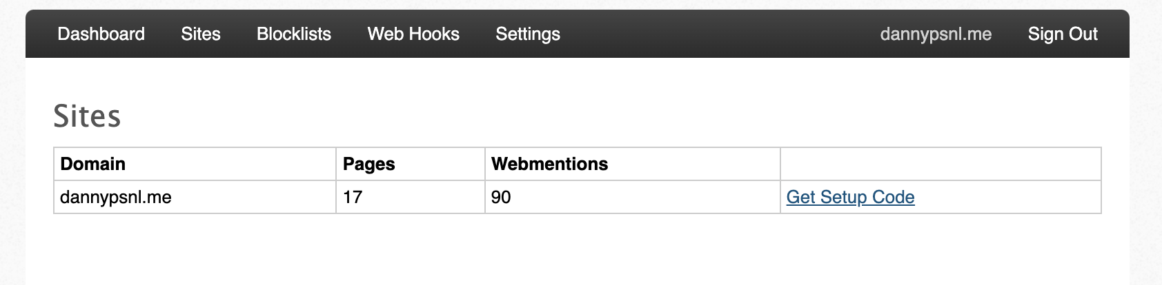
then send you a verify mail, after you login and click sites tab you will see a picture like
Click Get Setup Code, then you will see link like below
https://webmention.io/<domain>/webmention
that's the <endpoint> for your site. We need to put it into tree.xsl
If you want to send POST request to webmention.io manually, then here we already complete, but if you want to combine social media, we need to do more.
bridgy is a complex service, it plays several roles, but use it is relatively easy. At home page, you should see
I only use mastodon as example, you click the mastodon button, then get
click Cross-post to a Mastodon account..., unless your site is also a fediverse instance and know what to do. Then it would list your accounts (connected to bridgy) at Click to open an account you're currently logged into, go for one then you would see a form Enter post URL:, that's the place to give it your post link, but no rush, we need to prepare something.
First, we cannot use https://domain/xxx.xml (I open an issue for this)
and invoke \hentry{describe the tree} in every tree that you want to provide webmentions.
Now, your tree has proper content, the final step is using xsltproc
xsltproc default.xsl xxx.xml > xxx.html
to provide html version for post, then cross post html link on bridgy.
If all correct, you will be able to see the Dashboard of webmention.io has a list of reactions, which is made by people click like, repost, or reply your toot on mastodon. You might wondering do I missing something here? Yes, we want webmentions because we want to show reactions on our site, we will interact with webmention.io's APIs to collect mentions data, so that we can show them, that will be the next post.
Discuss how can we implement a webmention receiver for forester.
Each post in forester will be a xml (let's use my site as the example https://dannypsnl.me/xxx.xml), post should provide the following content in <head></head>
The receiver must check that source and target are valid URLs [URL] and are of schemes that are supported by the receiver. (Most commonly this means checking that the source and target schemes are http or https).
The receiver must reject the request if the source URL is the same as the target URL.
The receiver should check that target is a valid resource for which it can accept Webmentions. This check should happen synchronously to reject invalid Webmentions before more in-depth verification begins. What a "valid resource" means is up to the receiver. For example, some receivers may accept Webmentions for multiple domains, others may accept Webmentions for only the same domain the endpoint is on.
If the receiver is going to use the Webmention in some way, (displaying it as a comment on a post, incrementing a like counter, notifying the author of a post), then it must perform an HTTP GET request on source, following any HTTP redirects (and should limit the number of redirects it follows) to confirm that it actually mentions the target. The receiver should include an HTTP Accept header indicating its preference of content types that are acceptable.
If the Webmention was not successful because of something the sender did, it must return a 400 Bad Request status code and may include a description of the error in the response body.
However, hosting a receiver can be annoying, so the next post I will introduce how to build on the top of some existed tools.
theorem : ∀ {n} → (i j : Fin n) → (a : n Cups)
  ------------------------------------------------
  → χ ((a [ i ]%= _⁻¹) [ j ]%= _⁻¹) ≡ χ a
theorem i j a =
  begin
    χ (updateAt (updateAt a i _⁻¹) j _⁻¹) ≡⟨ lemma j (a [ i ]%= _⁻¹) ⟩
    χ (updateAt a i _⁻¹)⁻¹ ≡⟨ ⁻¹-selfInverse (sym (lemma i a)) ⟩
    χ a
  ∎ where open ≡-Reasoning
          open Lemma
其意義是,對任意有限多個杯子進行兩次翻轉,奇偶性不變。這個定理比實際遊戲進行的行為更廣泛一些,i ≢ j 才是對應現實中的翻杯子行為,因為選擇是先進行的,而翻轉是同時做。但因為對同一杯子翻轉兩次也不會改變奇偶狀態,所以 i ≡ j 也行。其中
module Lemma where
  lemma : ∀ {n} → (i : Fin n) → (a : n Cups)
    ----------------------------------------------------------
    → χ (a [ i ]%= _⁻¹) ≡ χ a ⁻¹
  lemma i a = {!  !}
---- MODULE plustwo ----
EXTENDS Integers

CONSTANT Limit

(* --algorithm plustwo
variables x = 0;
begin
    while x < Limit do
        x := x + 2;
    end while;
end algorithm; *)
\* BEGIN TRANSLATION (chksum(pcal) = "3f62e9ff" /\ chksum(tla) = "239a9ecd")
\* END TRANSLATION
=====
由 PlusCal 產出的不變量會被包在 BEGIN TRANSLATION 到 END TRANSLATION 裡面,可以發現它還會檢查 checksum。由於這個區塊內的程式會被機器生成的內容覆蓋,要記得千萬不要把自己寫的不變量放在這裡面。
上面的 CONSTANT Limit 可以在 model 的設定檔 .cfg 中指定,這是為了避免把常數寫死在 TLA+ 主程式中,好在檢查前可以進行修改。
但指令需要編碼才能被 CPU 讀取,因此會有一系列的數字與對應的指令,組合語言則是為了讓人類可以閱讀這些指令而設計的編碼,組譯器因此基本上只要直接把指令文字變成一連串數字即可!因此,可以看出組合語言確實是一種程式語言,而組譯器是最簡單的把語法變成數字語法的重寫系統,對應的計算系統則是電腦硬體執行的那個計算系統。
當然這省略了組譯器的模組化功能部分,不過這部分對理解組譯器的定位沒有什麼幫助。這部分是由被稱為 linker 的程式進行,把不同的物件檔連結起來,比較好的參考書籍有《Linker and Loader》
This is a smarter cd command. When I do z xxx, it would bring me to the most frequently used directory with "xxx" in the name. More you use it, it would get more accurated.
If \(M\) is closed term of ground type and \(\mathcal {C}\llbracket M \rrbracket = \mathcal {C}\llbracket V \rrbracket \) for a value \(V\), then \(M \Downarrow V\).
import http.server
import socketserver

PORT = 8000

handler = http.server.SimpleHTTPRequestHandler

with socketserver.TCPServer(("", PORT), handler) as httpd:
    print("Server started at localhost:" + str(PORT))
    httpd.serve_forever()
Then use command docker build . -t quiver-quiver:latest to create a docker image.
We use they via command kubectl apply -f ./quiver.yml.
Finally, you can go to http://k8s.orb.local and see you already run quiver tool on local machine. Other way is using traefik with docker compose, and goes to http://quiver.localhost.
The language of ∞-categories provides an insightful new way of expressing many results in higher-dimensional mathematics but can be challenging for the uninitiated. To explain what exactly an ∞-category is requires various technical models, raising the question of how they might be compared. To overcome this, a model-independent approach is desired, so that theorems proven with any model would apply to them all. This text develops the theory of ∞-categories from first principles in a model-independent fashion using the axiomatic framework of an ∞-cosmos, the universe in which ∞-categories live as objects. An ∞-cosmos is a fertile setting for the formal category theory of ∞-categories, and in this way the foundational proofs in ∞-category theory closely resemble the classical foundations of ordinary category theory. Equipped with exercises and appendices with background material, this first introduction is meant for students and researchers who have a strong foundation in classical 1-category theory.
@book{riehl_verity_2022,
      place={Cambridge},
      series={Cambridge Studies in Advanced Mathematics},
      title={Elements of ∞-Category Theory},
      DOI={10.1017/9781108936880},
      publisher={Cambridge University Press},
      author={Riehl, Emily and Verity, Dominic},
      year={2022},
      collection={Cambridge Studies in Advanced Mathematics}
}
We have product \(x \leftarrow 0 \rightarrow y\), and the \(y \to 1\) (terminal rule),
but complement \(x^\mathsf {c}\) existed and \(x + y\) has no need to be \(1\),
so somewhere between \(y \to 1\) has a \(x^\mathsf {c}\).
Proposition. \(x \sqsubseteq y\) if and only if \(y^\mathsf {c} \sqsubseteq x^\mathsf {c}\) [math-003N]
Boolean algebra can be encoded by indexing, for example, a venn diagram for two sets \(A, B\) divide diagram to four parts: \(1, 2, 3, 4\). Thus
\(A = \{1, 2\}\)
\(B = \{1, 3\}\)
\(A \cup B = \{1, 2, 3\}\)
\(A \cap B = \{1\}\)
\((A \cup B)^{\mathsf {c}} = \{4\}\)
The benefit of the encoding is the encoding let any sets can be treated as finite sets operation. So for any set check a boolean algebra is valid, indexing helps you check them by computer.
(define I (set 1 2 3 4))
(define A (set 1 2))
(define B (set 1 3))
(define ∅ (set))
(define ∩ set-intersect)
(define ∪ set-union)
(define (not S)
  (set-subtract I S))
(define (→ A B)
  (∪ (not A) B))
(define (- A B)
  (∩ A (not B)))
(define (≡ A B)
  (∪ (∩ A B) (∩ (not A) (not B))))
The proof use category language, \(\sqcap \) (product) and \(\sqcup \) (coproduct).
Assuming there have two complements \(y, z\) for an element \(x\), then \(x + y = x + z = 1\) and \(x \times y = x \times z = 0\).
By distributive law we have below diagram
Then we use \(x + y = x + z = 1\) to reduce it and get
Since there has at most one path, the diagram commute, hence \(y = z\).
The proposition says a space is Hausdorff if and only if its diagonal map \(\Delta : X \to X \times X\) to product space is closed, which given an alternative definition. Notice that close means its complement \(\Delta ^\mathsf {c}\) is open. The definition of \(\Delta \) is
The first direction is Hausdorff implies diagonal map is closed. Hausdorff means every two different points has a pair of disjoint neighborhoods \((U \in \mathcal {N}_x, V \in \mathcal {N}_y)\), where \(x \in U\) and \(y \in V\). therefore, every pair \((x, y)\) not line on the diagonal has \(U \times V\) cover them. The union of all these open sets \(U \times V\) indeed covers \(\Delta ^\mathsf {c}\), so the complement \(\Delta \) is closed.
The second direction is diagonal map is closed implies Hausdorff. Since
\[\Delta ^\mathsf {c} = \{(x, y) \mid x, y \in X (x \ne y) \}\]
is open, which implies for all \(x, y\) the pair \((x, y) \in \Delta ^\mathsf {c}\). Since \(\mathcal {N}_{(x, y)} = \mathcal {N}_x \times \mathcal {N}_y\), this implies the fact that \(\Delta ^\mathsf {c} \in \mathcal {N}_x \times \mathcal {N}_y\).
Also, for all \(U \in \mathcal {N}_x\) and \(V \in \mathcal {N}_y\), it's natural that \(U \times V \subseteq \Delta ^\mathsf {c}\), since the open set \(U \times V\) at most cover \(\Delta ^\mathsf {c}\).
Consider that reversely again, that means for all \((x, x) \in \Delta \), pair \((x, x) \notin U \times V\) (i.e. \(U \times V\) will not cover any part of diagonal), that implies \(U \cap V = \varnothing \) as desired.
To understand \(F\)-algebra, we will need some observations, the first one is we can summarize an algebra with a signature. For example, monoid has a signature:
\[ \begin {cases} 1 : 1 \to m \\ \cdot : m \times m \to m \end {cases} \]
or we can say ring is:
\[ \begin {cases} 0 : 1 \to m \\ 1 : 1 \to m \\ + : m \times m \to m \\ \times : m \times m \to m \\ - : m \to m \end {cases} \]
The next observation is we can consider these \(m\) as objects in a proper category \(C\), at here is a cartesian closed category. For example
monoid is a \(C\)-morphism \(1 + m \times m \to m\)
ring is a \(C\)-morphism \(1 + 1 + m \times m + m \times m + m \to m\)
Now, we generalize algebra's definition.
Definition. \(F\)-algebra (algebra for an endofunctor) [math-001L]
With a proper category \(C\) which can encode the signature of \(F(-)\), and an endofunctor \(F : C \to C\), the \(F\)-algebra is a triple: \[(F, x, \alpha )\] where \(\alpha : F \; x \to x\) is a \(C\)-morphism.
With the definition of \(F\)-algebra, we wondering if \(F\)-algebras of a fixed \(F\) form a category, and the answer is yes.
Definition. Category of \(F\)-algebras [math-001M]
The theorem actually proves the corresponding \(C\)-object \(i\) of initial algebra \((F, i, j)\) is a fixed point of \(F\). By reversing \(j\) with its inverse, we get a commute diagram below.
In Haskell, we are able to define initial algebra
newtype Fix f = Fix (f (Fix f))

unFix :: Fix f -> f (Fix f)
unFix (Fix x) = x
View \(j\) as constructor Fix, \(j^{-1}\) as unFix, then we can define m = alg . fmap m . unFix. Since m :: Fix f -> a, we have definition of catamorphism.
cata :: Functor f => (f a -> a) -> Fix f -> a
cata alg = alg . fmap (cata alg) . unFix
An usual example is foldr, a convenient specialization of catamorphism.
I mostly learn F-algebras from Category Theory for Programmers, and take a while to express the core idea in details with my voice with a lot practicing. The article answered some questions, but we always with more. What's an algebra of monad? What's an algebra of a programming language (usually has a recursive syntax tree)? Hope you also understand it well through the article and practicing.
If there exists \(B \xrightarrow {f} B\) such that \(f \circ b \ne b\) for all \(1 \xrightarrow {b} B\),
then there has no point-surjective morphism can exist for \(A \xrightarrow {g} B^A\).
Comma category is generated by two functors, denoted \((T \downarrow S)\).
To understand the idea, we can start from slice & co-slice category, which is a special case of comma category.
In co-slice category, we have objects \(\langle f, c \rangle \) where \(x \xrightarrow {f} c\), and morphism \(\langle f, c \rangle \xrightarrow {h} \langle f', c' \rangle \) where below diagram commutes:
We give another denotation \((x \downarrow C)\) for object \(x\) and its category \(C\) for this concept, and \((C \downarrow x)\) for the dual.
If we generalize the idea, by replacing category \(C\) with a functor \(S : D \to C\), then we get a category \((x \downarrow S)\) with
objects \(\langle f, d \rangle \) where \(x \xrightarrow {f} Sd\)
morphisms \(h : \langle f, d \rangle \to \langle f', d' \rangle \) where below diagram commutes:
If we replace object \(x\) to another functor \(T\)? It's the full picture of comma category:
現在考慮一個簽名
\[ f : (S \le A) \Rightarrow S \times S \to S \]
在 Java 裡面可以確實保證兩個參數跟回傳的型別都是同一個。在 Go 裡面這個簽名就只能寫成
\[ f : \hat P \times \hat P \to \hat P \]
而兩個參數跟回傳的型別不一定相同。現在我們就會發現乍看之下 interface 對類型的約束跟多型一樣可以被多個不同的型別滿足,但事實上根本就是不同的東西。
By introduce a indirect level of universe \(\mathcal {U}^-\), such that a subtype of normal universe \(\mathcal {U}\), and allows pattern matching.
By restricting it can only be used at inductive type definitions' dependent position, it preserves parametricity, solves the problem easier compare with subscripting universe.
In this setup, every defined type has type \(\mathcal {U}^-\) first, and hence
\(\mathbb {N} : \mathcal {U}^-\)
\(\mathbb {B} : \mathcal {U}^-\)
\(\mathbb {L} : \mathcal {U} \to \mathcal {U}^-\)
\(\mathbb {L}\) didn't depend on \(\mathcal {U}^-\), so we keep using tagless encoding to explain
data Term Type
  | ℕ => add (Term ℕ) (Term ℕ)
  | 𝔹 => eq (Term ℕ) (Term ℕ)
  | a => if (Term 𝔹) (Term a) (Term a)
  | a => lit a
We have \(\text {Term} : \mathcal {U}^- \to \mathcal {U}^-\), and then, if one wants List (Term Nat) it still work since \(\mathcal {U}^- \le \mathcal {U}\). But if one tries to define code below:
inductive Split Type^
  | Nat => nat
  | Bool => bool
  | _ => else

def id (A : Type) (x : A) : A =>
  match Split A
  | nat => 0
  | bool => false
  | _ => x
Since the \(\mathcal {U}\) isn't the subtype of \(\mathcal {U}^-\), program Split A won't type check, the definition will not work as intended.
This is indeed more boring than subscripting universe, but easier to check it does't break parametricity.
Till now, I haven't start to check the pattern of type, except the primitive exact value, if I'm going to push this further, a good example is:
inductive K Type^
  | List a => hi a
  | _ => he
This is quite intuitive since in implementation inductive types' head are also rigid values, just like constructors.
Int[+] is positive, Int[-] is negative.
The diagram in its syntactic category:
To ensure this, if the following syntax of each constructor c is a list of argument types Ti ..., we say the type of constructor of type T is Ti ... -> T[c]. The corresponding part is pattern matching's type rules will refine type T with the pattern matched constructor c, below marks all binder's refined type. The type T[c, ...] is a subtype of T.
def foo : Int -> Int
  | 0 => 0
  | + p =>
    -- p : Int[+, 0]
    p
  | - n =>
    -- n : Int[-, 0]
    n
def neg : Int -> Int
  | 0 => 0
  | + p => - (neg p)
  | - n => + (neg p)
We can see that the type information is squeezed, the second and third case need type casting. A potential solution is case type, and hence, neg has type like:
To extend this on to universe type Type, we say if there is an inductive family T
inductive T (xi : Xi) ...
  | ci Ti ...
  | ...
, there is a binding T : Xi ... -> Type[T]. As usual, Type[T, ...] is a subtype of Type. Therefore, in this configuration, writes down id : {A : Type} -> A -> A still has the only one implementation! And we can do type pattern matching if we have subscriptings. Consider
\(\mathcal {U}\) as Type
\(\mathbb {N}\) as Nat
\(\mathbb {B}\) as Bool
\(L\) as List
we have an example diagram as below
A motive example is the tagless encoding:
data Term Type
  | ℕ => add (Term ℕ) (Term ℕ)
  | 𝔹 => eq (Term ℕ) (Term ℕ)
  | a => if (Term 𝔹) (Term a) (Term a)
  | a => lit a
The final we can consider subtyping more, should we generally introduce subset of subscriptings as super type? In this setup then Type[Nat, Bool] <: Type[Nat] <: Type.
However, this is an over complicated idea, I prefer indirected universe more.
Element or member is a natural concept in set theory, one can use \(x \in A\) to denote \(x\) is an element of \(A\). We can extend the idea from view it in the category \(\bold {Sets}\):
Each element \(x\) of a set \(A\) corresponding to a function (set-morphism)
\[ \{\bullet \} \xrightarrow {x} A \]
Therefore, if we admit a category \(\mathcal {C}\) has a terminal object \(1\), we say an element \(x\) of object \(A \in Ob(\mathcal {C})\) is a morphism \(1 \xrightarrow {x} A\).
NOTE: A terminal object \(1\) has exact one morphism from elsewhere, therefore each \(1 \xrightarrow {x} A\) is a proper representation of a single element \(x \in A\).
If \(A \xrightarrow {f} B\) and \(A \xrightarrow {g} B\) are morphisms in the category \(\mathcal {C}\) then \(f = g\) if and only if for every object \(X\) and every morphisms \(X \xrightarrow {x} A\) we have \(f x = g x\)
The \(f = g\) leads to \(f x = g x\) is obvious.
Conversely, we already have \(f x = g x\) for all objects and morphisms. Let \(X = A\), by premise we got a commute diagram:
By diagram we got \(f = f \circ 1_A = g \circ 1_A = g\).
Pattern matching on type & following problems [tt-0001]
data Vec (A : Set a) : ℕ → Set a where
  []  : Vec A zero
  _∷_ : ∀ (x : A) (xs : Vec A n) → Vec A (suc n)
One can still try [] : Vec A 10, although the type check failed, it need a sophisticated unification check.
With Zhang's idea, we can do:
data Vec (A : Set a) : ℕ → Set a where
  zero => []
  suc n => _∷_ A (Vec A n)
Now, [] : Vec A n where \(n \ne 0\) is impossible to write down as usual, but now it's an easier unification!
Since there has no constructor [] for type Vec A n where \(n \ne 0\).
Another good example is finite set:
data Fin (n : N)
  | suc _ => fzero
  | suc n => fsuc (Fin n)
It requires overlapping pattern.
One more last, we cannot define usual equality type here (please check)
data Id (A : Type ℓ) (x : A) : A → Type ℓ where
  idp : Id A x x
Paper: Simpler indexed type essentially simplifies the problem of constructor selection just by turning the term-match-term problem to a term-match-pattern problem, which rules out numerous complication but also loses the benefit of general indexed types.
data Term : Set → Set1 where
  lit : ∀ {a} → a → Term a
  add : Term ℕ → Term ℕ → Term ℕ
  eq : Term ℕ → Term ℕ → Term 𝔹
  if : ∀ {a} → Term 𝔹 → Term a → Term a → Term a

eval : ∀ {a} → Term a → a
eval (lit x) = x
eval (add x y) = eval x + eval y
eval (eq x y) = eval x == eval y
eval (if c t e) with eval c
eval (if c t e) | true = eval t
eval (if c t e) | false = eval e
NOTE: There is a workaround in paper, and hence, the problem is inconvenience instead of impossible.
依此類推可以知道有 \(k\) 個單元建構子(即建構子 c 滿足 c : K )的型別 K 可以解釋為 \(k\)-type,接著 \(2 \to T\) 的元素應該有幾個呢?答案是 \(T \times T = T^2\),同理我們可以建立 \(k \to T = T \times ... \times T = T^k\) 的關係式。
依此可以建立一個簡單的直覺是 c : T 表示 \(+1\),而更加複雜的型別如 c : (2 -> T) -> T 就表示 \(+T^2\),建構子的參數表現了型別增長的速度,決定了型別的大小。
接著 foo (c foo) 就會陷入無限迴圈,為了要有強正規化,我們希望排除所有這類型的程式,比起一個一個去比對,直接禁止定義 c 這類的建構子可以更簡單的達成目的。Haskell/OCaml 的 data type 則不做此限制,因為它們不需要強正規化,這也是為什麼 dependent type 語言常説其 data type 是 inductive data type,並不輕易省略 inductive 這個詞,因為這樣定義的類型滿足 induction principle。
inductive Fib (a : Type) : Nat → Type where
| z : a → Fib a 0
| o : a → Fib a 1
| s : Fib a n → Fib a (n+1) → Fib a (n + 2)
可以看到 induction case 就是 \((2 \to F a) \to F a = {F a}^2 \to F a = F a \times F a \to F a\),所以對應的程式就是兩次呼叫 fib n + fib (n+1) 。當然,因為 fibonacci 還有一個利用矩陣計算的編碼
\[\begin {align} Expr &\to Term + Term \\ Term &\to Factor * Factor \\ Factor &\to Int \; | \; ( Expr ) \end {align}\]
這樣單調的修改在文法裡面確實很無聊,不過只要仔細觀察對應的 combinator,就會它們的型別發現這告訴了我們要怎麼利用 higher order function 來解決重複的問題!對 infix 運算形式(左結合)來說,通用的程式是
def infixL (op : Parsec (α → α → α)) (tm : Parsec α) : Parsec α := do
let l ← tm
match ← tryP op with
| .some f => return f l (← tm)
| .none => return l
這個 combinator 先解析左邊的 lower tm ,接著要是能夠解析 op 就回傳 op combinator 中存放的函數,否則就回傳左半邊的 tm 結果。使用上就像這樣
def infixL (opList : List (Parsec (α → α → α))) (tm : Parsec α)
: Parsec α := do
let l ← tm
let rs ← many do
for findOp in opList do
match ← tryP findOp with
| .some f => return (f, ← tm)
| .none => continue
fail "cannot match any operator"
return rs.foldl (fun lhs (bin, rhs) => (bin lhs rhs)) l
首先我們有一串 operator 而非一個,其次在右邊能被解析成 op tm 時都進行解析,最後用 foldl 把結果轉換成壓縮後的 α
我希望這次有成功解釋怎麼從規則對應到 parser combinator,所以相似的規則可以抽出相似的 higher order function 來泛化,讓繁瑣的規則命名變成簡單的函數組合。這個技巧當然不會只有在這裡被使用,只要遇到相似形的文法都可以進行類似的抽換,相似的型別簽名可以導出通用化的關鍵。
partial def infixR (opList : List (Parsec (α → α → α))) (tm : Parsec α)
: Parsec α := go #[]
where
go (ls : Array (α × (α → α → α))) : Parsec α := do
let lhs ← tm
for findOp in opList do
match ← tryP findOp with
| .some f => return ← go (ls.push (lhs, f))
| .none => continue
let rhs := lhs
return ls.foldr (fun (lhs, bin) rhs => bin lhs rhs) rhs
prefixop tm
def «prefix» (opList : List $ Parsec (α → α)) (tm : Parsec α)
: Parsec α := do
let mut op := .none
for findOp in opList do
op ← tryP findOp
if op.isSome then break
match op with
| .none => tm
| .some f => return f (← tm)
postfixop tm
def «postfix» (opList : List $ Parsec (α → α)) (tm : Parsec α)
: Parsec α := do
let e ← tm
let mut op := .none
for findOp in opList do
op ← tryP findOp
if op.isSome then break
match op with
| .none => return e
| .some f => return f e
In category theory, cone is a kind of natural transformation, to describe a diagram formally. The setup of cone is starting from a diagram, which we will define it as a category \(\mathcal {D}\) (usually is a finite one but no need to be) with two functors to the target category \(\mathcal {C}\). The two functors are
\(\Delta _c\) takes all objects of \(\mathcal {D}\) to a certain \(\mathcal {C}\)-object \(c\), and all morphisms to the identity \(1_c\)
\(F\) sends the diagram \(\mathcal {D}\) entirely into \(\mathcal {C}\)
The first functor is very clear, we always can do that for any category; the second functor will need \(\mathcal {C}\) has that diagram. Consider \(\mathcal {D}\) as below
If such diagram exists in \(\mathcal {C}\), then we have a proper way to define \(F\), there can have many such diagram in \(\mathcal {C}\), we denote them as \(\mathcal {C}(\mathcal {D})\). Now consider if there is a morphism from \(c\) to all objects in \(\mathcal {C}(\mathcal {D})\), that lift a natural transformation from \(\Delta _c \to F\).
We say \(c\) is an apex and the \(\mathcal {C}(\mathcal {D})\) is a plane in this sense, thus, such a natural transformation gives concept cone. With a fixed functor \(F\) (we also abuse language to say \(F\) is the diagram), varies \(\Delta _c\) bring different cones! When I get this, the picture in my mind is:
Image the head is apex and the body is the fixed diagram \(F\), you will also get the idea slowly.
To describe above idea, we make another category! By picking all apex of cone as objects, and picking morphism between apex in \(\mathcal {C}\) as morphisms, this is the category of cones (please check it does really a category).
With a fixed diagram \(\mathcal {D} \xrightarrow {F} \mathcal {C}\) and existing natural transformations \(\Delta _c \to F\), we get a category that consituited by
\(\Delta _c\) is a functor \(- \mapsto c : \mathcal {D} \to \mathcal {C}\) various on different \(c \in \mathcal {C}\).
objects: all cone objects \(c\) above the fixed diagram (via \(\Delta _c\) functor).
morphisms: \(\mathcal {C}\)-morphisms between cones.
Dual natural transformations \(F \xrightarrow {\beta } \Delta _c\) form cocones and a dual category.
The funny part we care here, is the terminal object of the category of cones, that is the next section.
A limit or universal cone is a terminal object of category of cones.
If you consider it carefully, and you will find this is the best cone of cones, because every other cones can be represented by composition of an addition morphism from itself to the limit!
Definition. Limit and colimit (universal cone and cocone) [math-002N]
With a fixed diagram \(\mathcal {D} \xrightarrow {F} \mathcal {C}\), a limit is a terminal of the category of cones, denoted as \(\lim _{\mathcal {D}} F\).
notice that we can freely abuse language and say a \(\mathcal {C}\)-diagram is a functor target to \(\mathcal {C}\)
Limit might not exist, so you have to ensure there has one.
The dual concept colimit is an initial of category of cocones, denoted as \(\underset {\mathcal {D}} {\text {colim}}F\).
With concept of cone and limit, you might already find there has some concept can be replaced by cone and limit, you're right and that would be fun to rewrite them in this new sense. Have a nice day.
在最上層的程式中,推導函數會直接被調用來得出 term 的 type,它會適當的調用 check 去檢查是否有型別錯誤
infer :: Env -> Ctx -> Raw -> M VTy
infer env ctx = \case
SrcPos pos t -> addPos pos (infer env ctx t)
Var x -> case lookup x ctx of
Just a -> return a
Nothing -> report $ "Name not found: " ++ x
U -> return VU
t :@ u -> do
tty <- infer env ctx t
case tty of
VPi _ a b -> do
check env ctx u a
return $ b $ eval env u
tty -> report $ "Cannot apply on: " ++ quoteShow env tty
Lam {} -> report "cannot infer type for lambda expression"
Pi x a b -> do
check env ctx a VU
check ((x, VVar x) : env) ((x, eval env a) : ctx) b VU
return VU
Let x a t u -> do
check env ctx a VU
let ~a' = eval env a
check env ctx t a'
infer ((x, eval env t) : env) ((x, a') : ctx) u
check :: Env -> Ctx -> Raw -> VTy -> M ()
check env ctx t a = case (t, a) of
(SrcPos pos t, _) -> addPos pos (check env ctx t a)
(Lam x t, VPi (fresh env -> x') a b) ->
-- after replace x in b
-- check t : bx
check ((x, VVar x') : env) ((x, a) : ctx) t (b (VVar x'))
(Let x a' t' u, _) -> do
check env ctx a' VU
let ~a'' = eval env a'
check env ctx t' a''
check ((x, eval env t') : env) ((x, a'') : ctx) u a
_ -> do
tty <- infer env ctx t
unless (conv env tty a) $
report (printf "type mismatch\n\nexpected type:\n\n \%s\n\ninferred type:\n\n \%s\n" (quoteShow env a) (quoteShow env tty))
SrcPos 這個情況只需要加上位置訊息之後往下 forward 即可
要是 term 是 lambda \(\lambda x . t\) 且 type 是 \(\Pi (x' : A) \to B\)
化簡函數就是把 term 變成 value 的過程,它只需要 environment 而不需要 context
eval :: Env -> Tm -> Val
eval env = \case
SrcPos _ t -> eval env t
Var x -> fromJust $ lookup x env
t' :@ u' -> case (eval env t', eval env u') of
(VLam _ t, u) -> t u
(t, u) -> VApp t u
U -> VU
Lam x t -> VLam x (\u -> eval ((x, u) : env) t)
Pi x a b -> VPi x (eval env a) (\u -> eval ((x, u) : env) b)
Let x _ t u -> eval ((x, eval env t) : env) u
SrcPos 一如既往的只是 forward
變數就是上環境尋找
\(\beta \)-reduction 的情形就是先化簡要操作的兩端,然後看情況
函數那頭是 lambda,就可以當場套用它的 host lambda 得到結果
這個情形比較有趣,有很多名字像是卡住、中性之類的描述,簡單來說就是沒辦法繼續化簡的情況。我們用 VApp 儲存這個結果,conversion check 裡面會講到怎麼處理這些東西
type Name = String
type Ty = Tm
type Raw = Tm
data Tm
= Var Name -- x
| Lam Name Tm -- \x.t
| Tm :@ Tm -- t u
| U -- universe
| Pi Name Ty Ty -- (x : A) -> B x
| Let Name Ty Tm Tm -- let x : A = t; u
{- helper -}
| SrcPos SourcePos Tm -- annotate source position
deriving (Eq)
執行會產出的語言的定義如下,可以看到 lambda 跟 \(\Pi \) 都運用了宿主環境的函數
type VTy = Val
data Val
= VVar Name
| VApp Val ~Val
| VLam Name (Val -> Val)
| VPi Name Val (Val -> Val)
| VU
type M = Either (String, Maybe SourcePos)
report :: String -> M a
report s = Left (s, Nothing)
addPos :: SourcePos -> M a -> M a
addPos pos ma = case ma of
Left (msg, Nothing) -> Left (msg, Just pos)
ma -> ma
quote :: Env -> Val -> Tm
quote env = \case
VVar x -> Var x
VApp t u -> quote env t :@ quote env u
VLam (fresh env -> x) t -> Lam x $ quote ((x, VVar x) : env) (t (VVar x))
VPi (fresh env -> x) a b -> Pi x (quote env a) $ quote ((x, VVar x) : env) (b (VVar x))
VU -> U
nf :: Env -> Tm -> Tm
nf env = quote env . eval env
fn main() -> Result<(), anyhow::Error> {
// 設定需要什麼能力
let config = ConfigBuilder::new(CommonConfigOptions::default())
.with_host_registration_config(HostRegistrationConfigOptions::default().wasi(true))
.build()?;
// 建立 import object,語意是從 host 引入名為 host_suffix 的函數
let import = ImportObjectBuilder::new()
.with_func::<(i32, i32), (i32, i32), !>("host_suffix", host_suffix, None)?
.build("host")?;
// 建立 vm 並註冊模組
let vm = Vm::new(Some(config))?
.register_import_module(import)?
.register_module_from_file("app", "app.wasm")?;
// 執行叫做 app 模組中名叫 start 的函數並查看結果
let result = vm.run_func(Some("app"), "start", None)?;
println!("result: {}", result[0].to_i32());
}
Host function 的定義如下
#[host_function]
fn host_suffix(caller: Caller, input: Vec<WasmValue>) -> Result<Vec<WasmValue>, HostFuncError> {
let mut mem = caller.memory(0).unwrap();
let addr = input[0].to_i32() as u32;
let size = input[1].to_i32() as u32;
let data = mem.read(addr, size).expect("fail to get string");
let mut s = String::from_utf8_lossy(&data).to_string();
s.push_str("_suffix");
// 總之 wasm 模組的記憶體肯定不會用到還不存在的位址
let final_addr = mem.size() + 1;
// 繼續增加一個 page size 的區塊
mem.grow(1).expect("fail to grow memory");
// 把要傳回去的字串寫入位址
mem.write(s.as_bytes(), final_addr)
.expect("fail to write returned string");
Ok(vec![
// 第一個回傳值是指標
WasmValue::from_i32(final_addr as i32),
// 第二個回傳值是長度
WasmValue::from_i32(s.len() as i32),
])
}
了解完 strictly positive 的必要性後,我們用例子來理解什麼是不一致的系統。這裏我假設讀者都已經知道 type as logic(program as proof) 是什麼,所以不再重複。第一個例子是 not-bad :
data Bad
bad : (Bad → Bottom) → Bad
notBad : Bad → Bottom
notBad (bad f) = f (bad f)
isBad : Bad
isBad = bad notBad
absurd : Bottom
absurd = notBad isBad
Bottom (\(\bot \)) 本來應該是不可能有任何元素的,即不存在 x 滿足 x : Bottom 這個 judgement,但我們卻成功的建構出 notBad isBad : Bottom 。如此一來我們的型別對應到的邏輯系統就有了缺陷。
data Term
abs : (Term → Term) → Term
app : Term → Term → Term
app (abs f) t = f t
w : Term
w = abs (λ x → app x x)
loop : Term
loop = app w w
loop 的計算永遠都不會結束,然而證明器用到的 dependent type theory 卻允許型別依賴 loop 這樣的值,因此就能寫出讓 type checker 無法停止的程式。換句話說,證明器仰賴的性質缺失。事實上 Term 跟 Bad 的問題就是違反了 strictly positive 的性質,或許也有人已經發現了兩者 constructor 型別的相似之處。接下來我們來看為什麼這樣的定義會製造出不一致邏輯。
根據這兩條規則,我們說 arrow types \(A \Rightarrow B\) 是 covariant in B 和 contravariant in A,或是說 A varies negatively 以及 B varies positively in \(A \Rightarrow B\)
For a tangent space \(T_pM\), covectors at the point \(p\) form a dual vector space as \(T_pM\), so called cotangent space of \(T_pM\), denotes \(T^*_pM\).
One can view a 1-form at least three different ways, let \(\alpha \) is a smooth 1-form, we have the following interpretations of \(\alpha \)
\(\alpha : M \to T^*M\) as definition, so that \(\alpha (-)\) takes points as arguments; \(\alpha (p) \in T^*_pM\), this also denotes \(\alpha _p = \alpha (p)\) sometimes.
\(\alpha : TM \to \R \) so that for \(v_p \in T_pM\) we make sense of \(\alpha (v_p)\) by \(\alpha (v_p) = \alpha _p(v_p)\).
\(\alpha : \mathfrak {X}(M) \to C^\infty (M)\) is a \(C^\infty (M)\)-linear map, where for \(X \in \mathfrak {X}(M)\) we interpret \(\alpha (X)\) as the smooth function
\[p \mapsto \alpha _p(X_p)\]
Let \(E_1, E_2, \dots , E_n\) be smooth vector fields defined on some open subset \(U \subseteq M\) of a smooth \(n\)-manifold \(M\). If \(E_1(p), E_2(p), \dots , E_n(p)\) form a basis for \(T_pM\) for each \(p \in U\), then we say \((E_1, E_2, \dots , E_n)\) is a moving frame or a frame field over \(U\).
Construct \(\text {rep} : M \to (M \to M)\) by currying \(\otimes \) \(\text {rep}(m) := \lambda m'. m \otimes m'\). This function is a monoid morphism, because
\(\text {rep}(I) = \lambda m. m = id\)
\[\begin {aligned} &\text {rep}(a \otimes b) = \lambda m'. (a \otimes b) \otimes m' \\ &= \lambda m'. a \otimes (b \otimes m') \\ &= (\lambda m. a \otimes m) \circ (\lambda n. b \otimes n) \\ &= \text {rep}(a) \circ \text {rep}(b) \end {aligned}\]
and it's an injection, since we can define \(\text {abs} : (M \to M) \to M\) such that
\[\text {abs}(k) = k(e)\]
so \(\text {abs}(\text {rep(m)}) = m \otimes e = m\).
A binoidal category is a category \(\mathbb {C}\) endowed with an object \(I \in \mathbb {C}\) and an object \(A \otimes B\) for each \(A, B \in \mathbb {C}\). There are functors
An effectful category is an identity-on-objects functor \(\color {blue}\mathbb {V}\color {black} \to \color {red}\mathbb {C}\color {black}\) from a monoidal category \(\color {blue}\mathbb {V}\color {black}\) (the pure morphisms, or "values") to a premonoidal category \(\color {red}\mathbb {C}\color {black}\) (the effectful morphisms, or "computations"), that strictly preserves all of the premonoidal structure and whose image is central.
this motivates us to find corresponding object of effects in premonoidal category, and uses the following additional (control) string to point out the order.
then ensure their tensor will coherence at the gold line. In Collages of String Diagrams they point out an usage of bimodular categories to model basic binary semaphore concept.
A nonzero element \(a\) of an integral domain \(D\) is called irreducible if \(a\) is not a unit and whenever \(b,c \in D\) with \(a = bc\), then \(b\) or \(c\) is a unit.
A sieve on the object \(U\) is a family of morphisms \(R\) that saturated in the sense that, \((V \xrightarrow {\alpha } U) \in R\) implies \((W \xrightarrow {\alpha \circ \beta } U) \in R\) for any \(W \xrightarrow {\beta } V\).
Let \(C\) be a small category. A Grothendieck topology on \(C\) is defined by specifying, for each object \(U \in C\), a set \(J(U)\) of sieves on \(U\), called covering sieves of the topology, such that
For any \(U\), the maximal sieve \(\{ \alpha \mid \fbox {?} \xrightarrow {\alpha } U \}\) is in \(J(U)\)
If \(R \in J(U)\) and \(V \xrightarrow {f} U\) is a morphism of \(C\), then the sieve
\[f^*(R) = \{ W \xrightarrow {\alpha } V \mid f\circ \alpha \in R \}\]
is in \(J(V)\)
If \(R \in J(U)\) and \(S\) is a sieve on \(U\) such that, for each \((V \xrightarrow {f} U) \in R\), we have \(f^*(S) \in J(V)\), then \(S \in J(U)\)
Let \(C\) be a small category with pullbacks. A Grothendieck pretopology on \(C\) is defined by specifying, for each object \(U \in C\), a set \(P(U)\) of families of morphisms of the form
\[\{ U_i \xrightarrow {\alpha _i} U \mid i \in I \}\]
called covering families of the pretopology, such that
For any \(U\), singleton set of the identity morphism \(\{ U \xrightarrow {1} U \}\) is in \(P(U)\).
If \(V \to U\) is a morphism in \(C\), and \(\{ U_i \to U \mid i \in I \}\) is in \(P(U)\), then the pullback \(\{ V \times _U U_i \xrightarrow {\pi _1} V \mid i \in I \}\) is in \(P(V)\).
If \(\{ U_i \xrightarrow {\alpha _i} U \mid i \in I \}\), and \(\{ V_{ij} \xrightarrow {\beta _{ij}} U_i \mid j \in J_i \}\) in \(P(U_i)\) for each \(i \in I\), then
\[\{ V_{ij} \xrightarrow {\alpha _i \circ \beta _{ij}} U \mid i \in I, j \in J_i \}\]
is in \(P(U)\).
Let \(S\) be an oriented regular surface, and let \(p \in S\). Let \(\partial _1, \partial _2\) be an orthonormal basis of \(T_pS\) with respect to which the Weingarten map is represented by a diagonal matrix
Let \(S\) be an oriented surface, let \(N : S \to \R ^3\) be a unit normal vector field on \(S\). Thus, \(N(p)\) only outputs an element of the sphere \(S^2 \subset \R ^3\), so \(N\) is also a function \(S \to S^2\). Such \(N\) is called the Gauss map.
The idea still work for higher dimension. Let \(S\) be an differentiable manifold with dimension \(n-1\), let \(N : S \to \R ^n\), then \(N : S \to S^{n-1} \subset \R ^n\).
A connection is compatible with the metric \(\langle -,- \rangle \) if for any smooth curve \(\gamma \) and any pair of parallel vector fields \(P\) and \(P'\) along \(\gamma \), we have
Let \(X\) and \(Y\) be two \(C^\infty \) tangent vectorfields on open set \(U\) of a differentiable manifold \(M\), the Lie bracket of \(X\) and \(Y\) is
\[[X,Y] := XY - YX\]
which takes two tangent fields and produces a new tangent field. The Lie derivative
\[L_XY = [X,Y]\]
Theorem. The Lie bracket is another tangent vector space [#329]
Let \(M\) be a \(n\)-dimensional \(C^\infty \)-manifold, \(q \in M\) and \(X_1, \dots , X_k\) be a list of linear independent \(C^\infty \)-vector fields, and \(1 \le k \le n\). Then if for all \(\alpha , \beta \)
\[[X_\alpha , X_\beta ] = 0\]
There exists \(C^\infty \)-immersion locally, i.e.
\[\lambda : U \subseteq \R ^k \looparrowright M\]
makes
\(q \in \lambda (U)\) and
\(X_\alpha = \frac {\partial \lambda }{\partial x^\alpha }\) for all \(\alpha \).
Let \(H\) be a normal subgroup of \(G\), the quotient group of \(G\) modulo \(H\) denoted \(G / H\), is the group \(G / \sim \) obtained from the relation \(\sim \) defined as
\[G / \sim \ = \{ aH \mid a \in G \} = \{ Ha \mid a \in G \}\]
In terms of cosets, the product in \(G / H\) is defined by
The left-cosets of a subgroup \(H\) in a group \(G\) are the sets \(aH\) for all \(a \in G\). The right-cosets of \(H\) are the sets \(Ha\) for all \(a \in G\).
Then \(A^i = \begin {bmatrix}a\\b\\c\end {bmatrix} = \delta ^i_j \begin {bmatrix}a\\b\\c\end {bmatrix} = \delta ^i_j A^j\). It's clear that this idea is general, even \(i, j\) have different dimensions, the form
Instead of denotes a vector as \(\vec {A}\), index form denotes \(A^\mu \), \(\mu \) is not exponent here, but index to each component. Let's take a concrete example, if \(A^\mu \) has dimension \(4\), then \(\mu = 0, 1, 2, 3\), thus
Let \(\mathbb {k}\) be a fixed field. A category \(C\) is called a \(\mathbb {k}\)-linear category if all hom-spaces are \(\mathbb {k}\)-vector spaces and the multiplication is bilinear. An object \(X \in C\) is a zero object if for all \(Y \in C\), we have \(\text {Hom}_{C}(X, Y) = \text {Hom}_{C}(Y, X) = 0\).
A functor between two \(\mathbb {k}\)-linear categories is call \(k\)-linear if the maps between the hom-spaces are \(\mathbb {k}\)-linear.
\(\text {VECT}(\mathbb {k})\), \(\text {vect}(\mathbb {k})\), \(\text {mat}(\mathbb {k})\) are examples of \(\mathbb {k}\)-linear categories. For any \(\mathbb {k}\)-algebra \(A\), we have \(\mathbb {k}\)-linear categories:
MOD-\(A\) The category of all right \(A\)-modules
Mod-\(A\) The category of all finitely generated right \(A\)-modules
mod-\(A\) The category of all finitely-dimensional right \(A\)-modules
The zero object in these categories is zero vector space with trivial \(A\)-action. The hom-spaces in these categories are often denoted by \(\text {Hom}_{A}(M, N)\). Respectively, for left modules we have \(A\)-MOD, \(A\)-Mod, and \(A\)-mod.
Due to functor can be viewed as diagonal functor that has dummy contravariant variable, we have a cool reuse of end notation. Let \(F, G : \mathcal {C} \to \mathcal {D}\) be functors, a natural transformation from \(F\) to \(G\) can be viewed as an end, and hence we have an isomorphism
A formula if arithmetic is said to be \(\Delta _0\) if it has no unbounded quantifiers. Alternatively, the set of \(\Delta _0\) formulas is the smallest set containing atomic formulas in the language of arithmetic and closed under boolean operations and bounded quantification.
The hierarchies of \(\Sigma _n\) and \(\Pi _n\) formulas are defined simultaneously and inductively as follows
\(\Sigma _0 = \Pi _0 = \Delta _0\)
If \(A \in \Sigma _n\), then \(A \in \Pi _{n+1}\)
If \(A \in \Pi _n\), then \(A \in \Sigma _{n+1}\)
If \(A \in \Sigma _{n+1}\), then \(\exists x A \in \Sigma _{n+1}\)
If \(A \in \Pi _{n+1}\), then \(\forall x A \in \Pi _{n+1}\)
Let \(M\) be a differentiable manifold with an affine connection \(\nabla \). There exists a unique correspondence which associates to a vector field \(V\) along the differentiable curve \(\gamma : [0,1] \to M\) another vector field \(\frac {DV}{dt}\) along \(\gamma \), called the covariant derivative of \(V\) along \(\gamma \).
Let \(M\) be a differentiable manifold with an affine connection \(\nabla \). A vector field \(V\) along a curve \(\gamma : [0,1] \to M\) is called parallel if for all \(t \in [0,1]\) its covariant derivative (Definition [math-00EO]) is zero, i.e.
\[\frac {DV}{dt} = 0\]
Definition. Diffeomorphism and local diffeomorphism [math-00BR]
Let \(\varphi : M \to N\) be a differentiable map, if \(d\varphi _p : T_p M \to T_{\varphi (p)} N\) is an isomorphism, then \(\varphi \) is a local diffeomorphism at \(p\).
Say \(M\), \(N\) has dimension \(m\), \(n\), respectively, then \(\varphi \) is an immersion implies \(m \le n\).
If \(\varphi \) is a homeomorphism onto \(\varphi (M) \subset N\), where \(\varphi (M)\) has the subspace topology induced from \(N\), then \(\varphi \) is an embedding, \(M\) is a submanifold of \(N\).
As the subdivision becomes finer and finer, curvature variees less and less each \(\Delta _i\), approaching the constant value \(\mathcal {K}_i\), and in its limit yields
A typed partial combinatory algebra is a partial applicative structure (Definition [math-00E1]) satisfying the following conditions
For all \(A, B \in |A|\), there is a \(k_{AB} : A \Rightarrow B \Rightarrow A\) such that
\[ \forall a.\ k \cdot a \downarrow , \quad \forall a,b.\ k \cdot a \cdot b = a \]
For all \(A, B, C \in |A|\), there is a \(s_{ABC} : (A \Rightarrow B \Rightarrow C) \Rightarrow (A \Rightarrow B) \Rightarrow (A \Rightarrow C)\) such that
\[ \forall f, g.\ s \cdot f \cdot g \downarrow , \quad \forall f,g,a.\ s \cdot f \cdot g \cdot a \simeq (f \cdot a) \cdot (g \cdot a) \]
An integral domain \(R\) is a principal ideal domain if every ideal has the form \(\langle a \rangle = \{ r \cdot a \mid a \in R \}\) for some \(a \in R\).
Theorem. \(F\) a field implies \(F[x]\) a principal ideal domain [math-00DZ]
Since \(g(x) \in I\), we have \(\langle g(x) \rangle \subseteq I\)
Let \(f(x) \in I\), we might write \(f(x) = g(x)q(x) + r(x)\), only two conditions can hold
\(r(x) = 0\)
or \(\deg r(x) < \deg g(x)\)
The second one can't be true because the degree of \(g(x)\) by definition is the minimum, therefore \(r(x) = 0\).
Thus, if a \(f(x) \in I\), it must has a form \(f(x) = g(x)q(x)\). This shows that \(I \subseteq \langle g(x) \rangle \)
Definition. Degenerate and non-degenerate (simplex) [math-00DW]
With a fixed simplicial set \(X\), a \(n\)-simplex \(x \in X_n\) is said to be degenerate if there is \(m\)-simplex \(y \in X_m\) (\(m < n\)) and a \(\alpha : [n] \to [m]\), such that \(\alpha ^* : X_m \to X_n\) satisfies
\[ x = \alpha ^*(y) \]
In words, if there exists a lower \(m\)-simplex and a map from that to this \(n\)-simplex, then this \(n\)-simplex is degenerate.
A \(n\)-simplex is said to be non-degenerate, if it's not degenerate.
Let \(\gamma : [a,b]\to \R ^2\) be a simple closed curve. For any \(p \in \R ^2 \setminus \gamma \) not on the curve, there is a family of vectors
\[ \overrightarrow {p \gamma (t)} \]
Take these vectors only by direction form a map \(f_p : [a,b] \to S^1\), and let \(W(p)\) be the degree of \(f_p\).
Consider a very close window, so \(\gamma \) is merely a line, then pick two points \(p_1\) and \(p_2\), such that makes \(|W(p_1) - W(p_2)| = 1\), this is possible because one covers the bottom half of \(S^1\) counterclockwise, the other covers the top half of \(S^1\) clockwise, therefore the difference exactly turned around.
Follow the orientation of \(\gamma \), move the window, can see \(p_1\) and \(p_2\) will not change the coverage at any point of \(\gamma \), and hence there are two path-connected components wrap \(\gamma \).
Finally, for any \(p\) not on the curve \(\gamma \), the shortest path to \(\gamma \) must touch a \(p_1\) or a \(p_2\) first! Thus, the curve indeed cut the plane to two components.
Thus, for most inputs \(\psi (t_1, t_2)\) is the unit vector from \(\gamma (t_1)\) to \(\gamma (t_2)\). Rest cases are defined to make this function is continuous.
Let \(\alpha _0 : [0,1] \to T\) be the line segment from \((a,a)\) to \((b,b)\)
and \(\alpha _1 : [0,1] \to T\) be the line segment from \((a,a)\) to \((a,b)\) to \((b,b)\)
Now, defines a homotopy from \(\alpha _0\) to \(\alpha _1\), parameterize middle-segments by \(s : [0,1] \to T\) as \(\alpha _s\) to be a continuously family, which means \((s,t) \mapsto \alpha _s(t)\) should be a continuous function from \([0,1] \times [0,1] \to T\).
For each \(s \in [0,1]\), use \(D(s)\) denote the degree of \(\psi \circ \alpha _s : [0,1] \to S^1\).
Use lemma 2 to prove \(D(s)\) is locally constant, this is obvious because each \(s\) should uniquely determined a segment, which leads to same degree (the degree of \(\psi \circ \alpha _s\)). therefore continuous on \([0,1]\).
\(D : [0,1] \to \R \) is integer-valued and continuous, \(D\) must be constant on \([0,1]\), so \(D(1) = D(0)\).
\(D(0)\) by definition is the defree of the unit tangent function of \(\gamma \), which equals to the rotation index of \(\gamma \); we cannot prove \(D(0) = 1 \text { or } -1\), but if we can prove below \(D(1) = 1 \text { or } -1\), we are able to say the proof is complete.
A free group \(F(A)\) on set \(A\) will be an initial object in \(\mathcal {F}^A\).
In category language, which means if \(F(A)\) is a free group on \(A\) if there is a set-function \(j : A \to F(A)\) such that, for all groups \(G\) and set-functions \(f : A \to G\), there exists a unique group homomorphism \(\varphi : F(A) \to G\) such that
commutes. Algebra: Chapter 0 proves free group exists for any set \(A\), with beautiful direction-hinted graph. Conclusionally, we can say a free group \(F(A)\) is constructed by
The elements are list of \(x \in A\) and \(x^{-1} \in A'\), e.g. \(x,y,z \in A\) then \([x, y, z^{-1}] \in F(A)\); the operation is concating lists, this is associative.
The empty list of element \(e = []\) is the identity of \(F(A)\); since \([] + w = w + [] = w\)
If \(w\) is reduced list (i.e. remove \(a^{-1} a\) pair), then the inverse of \(w\) is obtained by reversing the list, and replace \(a \in A\) by \(a^{-1} \in A'\) and \(a^{-1}\) by \(a\).
Take an example can be more clear: The inverse list of \([a,b^{-1}]\) is \([b, a^{-1}]\), concat them and reduce by step
\[ [a,b^{-1}, b, a^{-1}] = [a, a^{-1}] = [] \]
Indeed is the identity element \([]\).
A free abelian group \(F^{ab}(A)\) on set \(A\), means there is a set-function \(j : A \to F^{ab}(A)\) such that, for all abelian group \(G\) and set-functions \(f : A \to G\), there exists a unique group homomorphism \(\varphi : F^{ab}(A) \to G\) such that the following diagram commutes
Therefore, \(F^{ab}(A)\) is an initial object of the category of abelian groups \(Ab\).
A free \(R\)-module \(F^R(A)\) on a set \(A\) is an initial object in \(R\)-Mod. Since the category of abelian groups \(Ab\) is the category of \(\Z \)-modules \(\Z \)-Mod, it's natural to ask \(R^{\oplus A} \cong F^R(A)\)
Let \(F \subseteq \R ^n\) be a set of points in \(\R ^n\), the symmetry group of \(F\) in \(\R ^n\) is the set of all isometries of \(\R ^n\) that carry \(F\) onto itself. The group operation \(\cdot \) is function composition \(\circ \).
We need to show \(y_\beta ^{-1} \circ y_\alpha \) (reparameterize on \(TM\)) has positive determinant, whenever what determinant \(x_\beta ^{-1} \circ x_\alpha \) (reparameterize on \(M\)) has. Let's view reparameterizations as matrices, and by definition \(x_\beta ^{-1} \circ x_\alpha \) works on \(M\) part and \(d(x_\beta ^{-1} \circ x_\alpha )\) works on tangent vectors.
Thus, we can view the reparameterization matrix on \(TM\) as (fill zeros to fit the dimension)
Then we can see that \(y_\beta ^{-1} \circ y_\alpha \) must have positive determinant, since \(d(x_\beta ^{-1}\circ x_\alpha )\) will have the same determinant as \(x_\beta ^{-1}\circ x_\alpha \), so
if \(x_\beta ^{-1}\circ x_\alpha \) is non-orientable, then the big matrix will cancel the negative, so has positive determinant;
else it's orientable, then the big matrix directly has positive determinant.
The cofactor of an element \(a_{ij}\) of a matrix \(A\) is called \(a^{ij}\) and is defined as \((-1)^{i+j}\) times the determinant of the \((n-1) \times (n-1)\) matrix formed by eliminating from \(A\) the row and column that \(a_{ij}\) belongs to.
With definition of cofactor, we now can define
\[ \det (A) = \sum ^n_{j=1} a_{ij} a^{ij} \]
for any fixed \(i\). This recursively defines a determinant for any rank matrix.
Consider a Riemann metric \(g\) (use angle notation \(\langle -,- \rangle \)), it's a \(\begin {pmatrix}0 \\ 2\end {pmatrix}\) tensor (i.e. it takes two vectors and returns a real number). By definition, \(g\) is symmetric, and hence if use basis of tangent space \(\frac {\partial }{\partial x^i}\) as input vectors, form a symmetric matrix
\(g\) is symmetric, thus, \(O^{-1}gO = g_d\) is a diagonal matrix, now say if \(g_d = \text {diag}(g_1, g_2, \dots , g_n)\), then we pick
\[ D = \text {diag}(d_1, d_2, \dots , d_n) \]
such that \(d_i = \sqrt {\vert g_i \vert }\), then output diagonal matrix will only have \(1\) or \(-1\) as component on the diagonal line. If we choose \(O\) to let all \(1\) or all \(-1\) appear first, we call it the canonical form of metric \(g\). The canonical form is an orthonormal basis.
A metric is called a Minkowski metric if it's canonical form is \(\text {diag}(-1, 1, 1, 1)\) or \(\text {diag}(1, -1, -1, -1)\). The special relativity has such a metric for \(n = 4\).
The action is properly discontinuous if each \(p \in M\) has a neighborhood \(U\) such that \(U \cap \varphi _g(U) = \varnothing \) for all \(g \ne 1_G\)
W <- G.vertices
-- W 表示 working set
while W ≠ ∅
-- 1. 從 W 選出有最大 saturation 的頂點 u
-- 2. 選出不在鄰邊的顏色集合中,最小的顏色 c
color[u] <- c -- 3. 分配顏色 c 給 u
W <- W - {u} -- 從 W 中刪除 u
這個演算法還需要最大 saturation 的定義:
\[ \text {saturation}(u) = \{ c \;|\; \exists v. v\in \text {adjacent}(u) \;\text {and}\; \text {color}(v) = c \} \]
saturation 是一個集合,最大指的是該集合的大小, 所以 \(W\) 可以用 leftist tree 之類的結構來快速選出有最大 saturation set 的那個頂點
A unital commutative quantale is a symmetricmonoidal closed preorder \(\mathcal {V} = (V, \le , I, \otimes , \multimap )\) that has all joins \(\vee A\) exists for all \(A \subseteq V\). The empty join often denote as \(0 := \vee \varnothing \).
If the preorder is non-symmetric, we got non-commutative quantale obviously.
Let \(\cdot \) be given by application, if \(M \in \Lambda \) induces an operation in \([L \bowtie L, L]\) representing some \(f : L \times L \to L\) then \(\lambda xy. M(\text {pair}\ x\ y)\) induces the corresponding operation in \(L, L \Rightarrow L\); conversely, if \(N\) induces an operation in \([L, L \Rightarrow L]\), then \(\lambda z. N (\text {fst}\ z) (\text {snd}\ z)\) induces the corresponding one in \([L \bowtie L, L]\).
Kleene's first model \(\mathcal {K}_1\) is a computability model consists of
the single datatype \(\N \)
operations are Turing computable partial functions \(\N \rightharpoonup \N \)
The model has standard products, the computable operation
\[ \langle m,n \rangle = (m+n)(m+n+1)/2 + m \]
defines a bijection \(\N \times \N \to \N \) and satisfied weak product. Any element \(i \in \N \) may serve as a weak terminal, because \(\Lambda n. i\) is computale.
Here \(\N \Rightarrow \N \) can only be \(\N \), so need a suitable operation \(\cdot : \N \times \N \to \N \). Let \(T_0, T_1, \dots \) be some chosen enumeration of all Turing machines for computing partial functions \(\N \rightharpoonup \N \), then there is a Turing machine that accepts two inputs \(e, a\) and returns the result of applying the machine \(T_e\) to the single input \(a\).
The partial functions \(f : \N \times \N \rightharpoonup \N \) representable within the model via the standard product operations are just the partial computable ones. We may also see that these coincide exactly with those represented by some total computable \(\tilde {f} : \N \to \N \), in the sense that \(f(c,a) \simeq \tilde {f}(c) \cdot a\) for all \(c,a \in \N \).
One half of this is immediate: given a computable \(\tilde {f}\) the operation \(\Lambda (c,a). \tilde {f}(c) \cdot a\) is computable. The other half is precisely the content of Kleene's s-m-n from basic computability theory: for any Turing machine \(T\) accepting two arguments, there is a machine \(T'\) accepting one argument such that for each \(c\), \(T'(c)\) is an index for a machine computing \(T(c,a)\) from \(a\).
A computability model \(\mathbb {C}\) has weak (binary cartesian) products if there is an operation assigning to each \(A,B \in \vert \mathbb {C} \vert \) a datatype \(A \bowtie B \in \vert \mathbb {C} \vert \) along with operations \(\pi _A \in \mathbb {C}[A \bowtie B, A]\) and \(\pi _B \in \mathbb {C}[A \bowtie B, B]\), such that for any \(f \in C[C,A]\) and \(g \in \mathbb {C}[C,B]\), there exists \(\langle f,g \rangle \in \mathbb {C}[C, A \bowtie B]\) satisfying the following for all \(c \in C\).
A higher-order structure is a computability model \(C\) possessing a weak terminal \((I,i)\), and endowed with the following for each \(A, B \in \vert C \vert \)
a choice of datatype \(A \Rightarrow B \in \vert C \vert \)
a partial function \(\cdot _{AB} : (A \Rightarrow B) \times A \rightharpoonup B\) (external to the structure of \(C\)).
The weak terminal picks out a subset \(A^\#\) for each \(A \in |C|\), namely the set of elements of the form \(f(i)\) where \(f \in C[I, A]\) and \(f(i) \downarrow \).
A higher-order (computability) model is a higher-order structure \(C\) satisfying the following conditions for some (or equivalently any) weak terminal \((I,i)\)
A partial function \(f : A \rightharpoonup B\) is present in \(C[A,B]\) iff there exists \(\hat {f} \in C[I, A \Rightarrow B]\) such that
\[\hat {f}(i) \downarrow , \quad \forall a \in A. \ \hat {f}(i) \cdot a \simeq f(a)\]
For any \(A,B \in \vert C \vert \), there exists \(k_{AB} \in (A \Rightarrow B \Rightarrow A)^\#\) such that
\[\forall a. \ k_{AB} \cdot a \downarrow , \quad \forall a,b. \ k_{AB} \cdot a \cdot b = a\]
For any \(A,B,C \in \vert C \vert \), there exists
\[s_{ABC} \in ((A \Rightarrow B \Rightarrow C) \Rightarrow (A \Rightarrow B) \Rightarrow (A \Rightarrow C))^\#\]
such that
\[\forall f,g. \ s_{ABC} \cdot f \cdot g \downarrow , \quad \forall f,g,a. \ s_{ABC} \cdot f \cdot g \cdot a \simeq (f \cdot a) \cdot (g \cdot a)\]
The Möbius strip (plane model) can be defined as a quotient topology of \([0, 1] \times (-1, 1)\) with usual \(\R \) metric, the equivalence relation is defined as
\[(0, s) \sim (1, -s)\]
Definition. Convergence (in topological space) [math-00CO]
Let \((a_n)_{n\in \N }\) be a sequence of a topological space \(X\), we say it converges to \(a \in X\) if for all neighborhoods \(N_a\) of \(a\), there is a \(N \in \N \) let all \(a_k \in N_a\) for all \(k \ge N\).
Every \((b, \infty )\) with \(b < 0\) is a neighborhoods of \(0\), and all points of the sequence are in it, so \((a_n)\) converges to \(0\).
However, every \((b, \infty )\) with \(b < -1\) is a neighborhoods of \(-1\), and all points of the sequence are in it, so \((a_n)\) also converges to \(-1\).
The argument can work on every \(b \in \R \) if \(b < 0\), so not every topological space can work with usual convergence definition that generalized from metric space, leads us to define Hausdorff.
A prime ideal \(A\) of a commutative ring \(R\) is a proper ideal of \(R\) such that \(a,b \in R\) and \(a \cdot b \in A\) imply \(a \in A\) or \(b \in A\).
A maximal ideal of a commutative ring \(R\) is a proper ideal of \(R\) such that, whenever \(B\) is an ideal of \(R\) and \(A \subseteq B \subseteq R\), then \(B = A\) or \(B = R\).
Take \([x]_\sim \) and \([y]_\sim \) in \(P^n(\R )\) with \([x]_\sim \ne [y]_\sim \).
Take open neighborhoods \(U, V \subseteq S^n\) of \(x\) and \(y\), respectively,
with \(U \cap V = -U \cap V = -U \cap -V = U \cap -V = \varnothing \).
It's always possible, since \(U\) and \(V\) are open curves on \(S^n\).
Then, such \(U \cup -U\) and \(V \cup -V\) are proper disjoint corresponded neighborhoods, for any two points \([x]_\sim \) and \([y]_\sim \) there are two disjoint neighborhoods.
Thus, \(P^n(\R )\) is Hausdorff.
Theorem. Residue integral domains/fields [math-00CN]
A nonempty set \(S\) of a ring \(R\) is a subring if \(S\) is closed under subtraction and multiplication. Which means \(a - b \in S\) and \(a \cdot b \in S\) should hold for all \(a, b \in S\).
Let \(A\) be a frame, its elements are opens. Let \(X\) be a set, its elements are points. Let \(\vDash \) be a subset of \(X \times A\), if \((x,a) \in \ \vDash \) then we write \(x \vDash a\) and say \(x\) satisfies \(a\). \((X,A,\vDash )\) is a topological system if
if \(S\) is a finite subset of \(A\)
\[x \vDash \bigwedge S \iff x \vDash a \text { for all } a \in S\]
if \(S\) is any subset of \(A\)
\[x \vDash \bigvee S \iff x \vDash a \text { for some } a \in S\]
Let \(\Gamma \) be a finite set of alphabets, \(M\) be a single datatype of memory states. A memory state is a function \(m : \Z \to \Gamma \). Any Turing machine \(T\) can be regarded as computing a certain partial function \(f_T : M \rightharpoonup M\) in the way: \(f_T(m) = m'\) if the execution of \(T\) with initial state \(m\), eventually halts yielding the final memory state \(m'\).
The model \(T_2\) consisting of the single datatype \(\N \) together with all Turing-computable partial functions \(\N \rightharpoonup \N \). This model needs some convention for representing natural numbers via memory states.
The model \(T_3\) conceptually have a read-only input tape, a write-only output tape, and a working tape that permits both reading and writing. The input and output tapes are functions \(d : \N \to \Gamma \), \(D\) is the set of all such total functions. Thus, the model consisting of the single datatype \(D\) and all machine-computable partial functions \(f : D \rightharpoonup D\).
Definition. Simulation of computability models [math-00CJ]
Let \(C\) and \(D\) be computability models with types indexed by \(T, U\) respectively. A simulation \(\gamma \) of \(C\) in \(D\) (denotes \(C \triangleright D\)) consists of
a mapping associating each type \(\tau \in T\) a representing type \(\gamma \tau \in U\);
for each \(\tau \in T\), a relation \(\Vdash ^\gamma _\tau \) between elements of \(D(\gamma \tau )\) and those of \(C(\tau )\).
subject to the following conditions
For each \(\tau \in T\) and each \(a \in C(\tau )\), there is some \(a' \in D(\gamma \tau )\) such that \(a' \Vdash ^\gamma _\tau a\).
Every operation \(f \in C[\sigma , \tau ]\) is tracked by some \(f' \in D[\gamma \sigma , \gamma \tau ]\), i.e. if \(f(a)\) is defined and \(a' \Vdash ^\gamma _\tau a\), then \(f'(a')\) is defined and \(f'(a') \Vdash ^\gamma _\tau f(a)\).
By definition of \(T_2\), a simulation \(T_2 \triangleright T_1\) is given. If \(n \in \N \) and \(m\) is a memory state, we take
\[m \Vdash n\]
iff \(m\) represents \(n\) in the sense we have defined. Every operation in \(T_2\) is tracked by one in \(T_1\).
We cannot have a simulation \(T_1 \triangleright T_2\), because there are uncountably many memory states. But there is a simulation for variant of \(T_1\), by restricting \(T_1\)'s memory states to those with a designated blank symbol in all but finitely many cells. Such memory states can be coded as natural numbers, and the action of any Turing machine may then be emulated by a partial computable function \(\N \rightharpoonup \N \). We thus obtain a simulation \(T_1^\text {fin} \triangleright T_2\).
We can simply found since \(\mu \) is \(C^\infty \), each partial differential of it still \(C^\infty \), and \(L_{a^{-1}}(b)\) is the inverse function share the same form and hence also \(C^\infty \), concludes that \(L_a\) is a diffeomorphism.
The determinant function \(\det : \R ^{n\times n} \to \R \) is continuous, \(GL(n, \R )\) is an open subset of \(\R ^{n\times n}\), with the standard topology on \(\R ^{n\times n}\).
hold for all \(n\). And then, instead of \(s_n = 0 \vee s_n = 1 \quad =\quad \text {true}\), we interpret \(s_n = 0 \vee s_n = 1\) as the \(n\)-th bit has now been read. Thus, we have
A real \(C^\alpha \)-premanifold is a locally \(\R \)-ringed space \((M, \mathcal {O}_M)\) with an open covering
\[ M = \bigcup _{i \in I}U_i \]
such that for all \(i \in I\) there exist \(m \in \N \), an open \(Y \subseteq \R ^m\), and an isomorphism of locally \(\R \)-ringed spaces \((U_i, {\mathcal {O}_M}_{\rvert {U_i}}) \cong (Y, \mathcal {C}^\alpha _Y)\) (called chart).
The differential of map \(\varphi \) at \(p\) is a map of tangent vectors \(T_p M \to T_{\varphi (p)} N\)
Let \(M, N\) be differentiable manifolds (\(m\) and \(n\) dimensional, resp) and let \(\varphi : M \to N\) be a differentiable mapping (Definition [math-00CB]). For every \(p \in M\) and for each \(v \in T_p M\), choose a differentiable curve \(\alpha : (-\epsilon ,\epsilon ) \to M\) with \(\alpha (0) = p\), \(a'(0) = v\). Take \(\beta = \varphi \circ \alpha \). The linear mapping
\[\begin {aligned} &d \varphi _p &:& &T_p M \to T_{\varphi (p)} N \\ &d\varphi _p(v) &=& &\beta '(0) \end {aligned}\]
is called the differential of \(\varphi \) at \(p\).
Proposition. The choice of curve is irrelevant [#439]
Let \(C,D\) be two categories. Given two functors \(P, Q : C^{op} \times C \to D\) a dinatural transformation \(\alpha : P \multimap Q\) consists of a family of morphisms
\[ \alpha _c : P(c,c) \to Q(c,c) \]
indexed by the objects \(c \in C\) and such that for any \(f : c \to c'\) the following diagram commutes
Definition. Rotation index of curve on plane (or degree of curve) [math-00C5]
Let \(\gamma : [a,b] \to \R ^2\) be a regular closed curve on plane \(\R ^2\), then there exists a smooth function \(\theta : [a,b] \to \R \) such that for all \(t \in [a,b]\), the unit tangent vector satisfies
If \(f : [a,b] \to S^1\) is a continuous function with \(f(a) = f(b)\), then there exists a continuous angle function \(\theta : [a,b] \to \R \) such that for all \(t \in [a,b]\)
\[ f(t) = (\cos \theta (t), \sin \theta (t)) \]
This function is unique up to adding an integer multiple of \(2\pi \).
Let \(f_1, f_2 : [a,b] \to S^1\) be continuous functions with \(f_1(a) = f_2(b)\) and \(f_2(a) = f_2(b)\). If \(f_1\) and \(f_2\) have different rotation indicies (Definition [math-00C5]), then exists \(t_0 \in [a,b]\) satisfies
since \(\delta \) has a net change of at least \(2\pi \), there must be an odd integer \(n\) multiple \(n\pi \) between \(\delta (a)\) and \(\delta (b)\). The intermediate value theorem implies that \(\delta \) achieves this value for some \(t_0 \in [a,b]\), so \(f_1(t_0) = -f_2(t_0)\).
The idea behinds this is two angles will be exactly be oppsite place on \(S^1\) at some point \(t_0\).
Definition. Ringed spaces and locally ringed spaces [math-00C3]
An \(R\)-ringed space is a pair \((X, \mathcal {O}_{X})\), where \(X\) is a topological space and where \(\mathcal {O}_{X}\) is a sheaf of commutative \(R\)-algebras on \(X\). The sheaf of rings \(\mathcal {O}_{X}\) is called the structure sheaf of \((X,\mathcal {O}_{X})\).
A locally \(R\)-ringed space is an \(R\)-ringed space \(X,\mathcal {O}_{X}\) such that for each point \(x \in X\), the stalk (Definition [math-00B5]) \(\mathcal {O}_{X,x}\) is a local ring. We then denote
by \(\mathfrak {m}_x\) the maximal ideal of \(\mathcal {O}_{X,x}\)
and by \(\kappa (x) := \mathcal {O}_{X,x} / \mathfrak {m}_x\) its residue field.
Proposition. A connected graph is a tree iff for each subgraph exists a point with degree 0 or 1 [math-00C2]
(\(\Longrightarrow \)) First, we only need to consider connected subgraph, since \(T\) is a tree. Then for any subgraph we can inherit tree order from the tree, then form a subtree and hence has leaf (with degree 1) or has a single point (with degree 0).
(\(\Longleftarrow \)) Suppose \(T\) is not a tree, which means it has a cycle, then we pick that cycle as subgraph, and that's contradict to the condition, and hence \(T\) is a tree.
Strictly positive types are those types which can be formed using \(0, 1, +, \times , \to , \mu , \nu \) with the restriction that types on the left hand side of the arrow have to be closed with respect to type variables. So, a strictly positive type in \(n\) variables is a type expression (with type variables \(X_1, \dots , X_n\)) by the following rules inductively
if \(K\) is a constant type then \(K\) is strictly positive.
each type variable \(X_i\) is strictly positive.
if \(F,G\) are strictly positive, then so are \(F + G\) and \(F \times G\).
if \(K\) is a constant type and \(F\) is strictly positive, then \(K \to F\) is strictly positive.
if \(F\) is a strictly positive type with \(n+1\) variables, then \(\mu X. F\) and \(\nu X. F\) are strictly positive types in \(n\) variables.
and non-inductive strictly positive type means the expression has no any \(\mu \) and \(\nu \) involved.
The central insight of the paper is all strictly positive types can be represented as containers.
This function is a minimal example that concurrency might not able to do it:
||
true
false
\(\bot \)
true
true
true
true
false
true
false
\(\bot \)
\(\bot \)
true
\(\bot \)
\(\bot \)
If a concurrency process is actually do by time sharing with the only unit, it might fall into a loop at one side and never check another computation, and hence cannot have the same semantic.
Let \(X = V(f_i)_{i\in I}\), each \(f_i(x, x) = 0\). Let \(g(x) = f_i(x,x)\) for some \(i\). Since Proposition [math-00BP] we have \(g(1) = f_i(1,1) = 0\), implies \((1,1) \in X\), leads to contradiction. Thus, \(X\) is not an affine variety.
Let \(R = V(f_i)_{i\in I}\), each \(f_i(x, y) = 0\). We can write \(f_i\) in form
\[ f_i = \sum _{j = 0}^2 g_j(y) x^j \]
since all \(x\in \R \) are included, and hence \(g_j\) are forced to be zero functions, and hence are zero polynomials. Which force \(R\) to include all \(y\in \R \) in \(R\), leads to contradiction. Thus, \(R\) is not an affine variety.
Proposition. Zero polynomial iff zero function when the field is infinite [math-00BP]
This proposition is helpful when we are going to show a set is not a variety.
Let \(k\) be an infinite field and let \(f \in k[x_1, \dots , x_n]\) be a polynomial. Then \(f = 0\) in \(k[x_1, \dots , x_n]\) if and only if \(f : k^n \to k\) is the zero function.
The zero polynomial's coefficients are all zero, so if direction is clear. The converse part can be show by induction on the number of variables \(n\):
When \(n = 1\), a nonzero polynomial in \(k[x]\) of degree \(m\) has at most \(m\) distinct roots. For the particular \(f\), \(f(a) = 0\) is assumed for all \(a \in k\). Since \(k\) is infinite, we just show \(f\) get infinitely many roots, and hence \(f\) must be the zero polynomial.
Assume converse is true for \(n-1\), and let \(f \in k[x_1,\dots ,x_n]\) be a polynomial that vanishes at all points of \(k^n\). By collecting the various powers of \(x_n\), \(f\) can be wrote in the form
where \(g_i \in k[x_1,\dots ,x_{n-1}]\). We will show that each \(g_i\) is the zero polynomial in \(n-1\) variables, which will force \(f\) to be the zero polynomial in \(k[x_1, \dots , x_n]\).
If we fix \((a_1, \dots , a_{n-1}) \in k^{n-1}\), we get the polynomial \(f(a_1, \dots , a_{n-1}, x_n) \in k[x_n]\). By our hypothesis on \(f\), this vanishes for every \(a_n \in k\). It follows from the case \(n=1\) that \(f(a_1, \dots , a_{n-1}, x_n)\) is the zero polynomial in \(k[x_n]\).
Use the above formula of \(f\), we see that the coefficients of \(f(a_1,\dots ,a_{n-1},x_n)\) are \(g_i(a_1, \dots ,a_{n-1})\), and thus \(g_i(a_1,\dots ,a_{n-1}) = 0\) for all \(i\). Since \((a_1,\dots ,a_{n-1})\) was arbitrarily chosen in \(k^{n-1}\), it follows that each \(g_i\) gives the zero function on \(k[x_1, \dots , x_{n-1}]\). Our inductive assumption then implies that each \(g_i\) is the zero polynomial in \(k[x_1, \dots , x_{n-1}]\). This force \(f\) to be the zero polynomial in \(k[x_1,\dots ,x_n]\) and completes the proof.
A differentiable manifold of dimension \(n\) is a set \(M\) and a family of injective mappings \(x_\alpha : U_\alpha \subset \R ^n \to M\) of open sets \(U_\alpha \) of \(\R ^n\) into \(M\) such that
\(\bigcup _\alpha x_\alpha (U_\alpha ) = M\)
for any pair \(\alpha , \beta \) with \(x_\alpha (U_\alpha ) \cap x_\beta (U_\beta ) = W \ne \varnothing \), the sets \(x_\alpha ^{-1}(W)\) and \(x_\beta ^{-1}(W)\) are open sets in \(\R ^n\) and the mappings \(x_\beta ^{-1} \circ x_\alpha \) and \(x_\alpha ^{-1} \circ x_\beta \) are differentiable.
The family \(\{ (U_\alpha , x_\alpha ) \}\) is maximal relative to the conditions (1) and (2).
A family \(\{ (U_\alpha , x_\alpha ) \}\) is called a differentiable structure on \(M\).
Proposition. Product of differentiable manifold [math-00BO]
Let \(M\) and \(N\) be differentiable manifolds (Definition [math-00BN]), and let \(\{ (U_\alpha ,x_\alpha ) \}\), \(\{ (V_\beta ,y_\beta ) \}\) be differentiable structures respectively. A mapping \(z_{\alpha \beta }(p,q) = (x_\alpha (p), y_\beta (q))\) for all \(p \in U_\alpha \) and \(q \in V_\beta \), then \(\{ (W_{\alpha \beta }, z_{\alpha \beta }) \}\) is a differentiable structure on \(M \times N\).
We need two parts: covering and differentiable to show it.
First we need to show \(\{ (U_\alpha \times V_\beta , z_{\alpha \beta }) \}\) covers \(M \times N\), by
\[ \bigcup _{\alpha \beta } z_{\alpha \beta }(U_\alpha \times V_\beta ) = \bigcup _{\alpha \beta } (x_\alpha (U_\alpha ), y_\beta (V_\beta )) = \bigcup _\alpha x_\alpha (U_\alpha ) \times \bigcup _\beta y_\beta (V_\beta ) \]
so the \(M \times N\) is covered by definition componentwise.
Then we are going to show for any \(\alpha \beta \) and \(\gamma \delta \), with
\(z_{\alpha \beta }(W_{\alpha \beta }) \cap z_{\gamma \delta }(W_{\gamma \delta }) = Z \ne \varnothing \),
the mappings \(z^{-1}_{\alpha \beta }(Z)\) and \(z^{-1}_{\gamma \delta }(Z)\) are open sets.
Consider \(z^{-1}_{\alpha \beta }(Z) = (x^{-1}_\alpha (Z), y^{-1}_\beta (Z))\), each component is open by definition, so immediately tell us \(z^{-1}_{\alpha \beta }(Z)\) is open in the induced product topology. The same argument can be applied to \(z^{-1}_{\gamma \delta }(Z)\).
Finally, we need to show \(z_{\gamma \delta }^{-1} \circ z_{\alpha \beta }\) and \(z_{\alpha \beta }^{-1} \circ z_{\gamma \delta }\) are differentiable, again by symmetry we only need to do it once:
\[ (z_{\gamma \delta }^{-1} \circ z_{\alpha \beta })(W_{\alpha \beta }) = (x_\gamma ^{-1} \circ x_\alpha (p), y_\delta ^{-1} \circ y_\beta (q)) \]
and components are differentiable by definition, so we get a differential of \(z_{\gamma \delta }^{-1} \circ z_{\alpha \beta }\) by taking differential componentwise.
Let \(k\) be a field, and let \(f_1, \dots , f_s\) be polynomials in \(k[x_1, \dots , x_n]\) (or \(k[\underline {x}]\) for short). Then an affine variety
\[ V(f_1, \dots , f_s) = \{ (a_1, \dots , a_n) \in k^n \mid f_i(a_1,\dots ,a_n)=0 \text { for all } 1 \le i \le s \} \]
is the set of all solutions of the system of equations
The idea is imaging there are \(p\)-points circles, each point has a color picked from \(a\) colors.
There are exactly \(a^p\) possible circles, now we group circles that isomorphic under rotation together, we can see that at most \(p\) circles each group.
Now, a \(p\)-points circles group can only have \(p\) elements or it has \(1\) elements, because no pattern can repeated in \(p\)-points.
Then we already complete, we can separate \(a^p\) many circles to \(N\) groups, each with \(p\) circles, and remains \(a\) circles are single colored.
Definition. Riemann manifold and Riemann metric [math-00BI]
whether \(s(\gamma _0) \gt s(\gamma _1)\) or \(s(\gamma _0) \lt s(\gamma _1)\), we know it doesn't make sense to use \(\gamma _0\) (or \(\gamma _1\)) to be shortest path, and hence one of \(d(p,q)\) and \(d(q,p)\)'s definition is wrong, so \(d(p,q) = d(q,p)\) has to be hold.
but notice that \(\gamma _1\) after \(\gamma _0\) is also a curve from \(p\) to \(q\), and \(\gamma _2\) by definition is one of the path with shortest length, and hence the length of \(\gamma _1\) plus \(\gamma _0\) at less equals to the length of \(\gamma _2\), or be bigger.
For two elements \(g,h \in G\) of a group \(G\), the conjugation \(g^h = h^{-1} g h\). This can be applied to a subset \(A \subseteq G\), by \(A^k = \{ a^k \mid a \in A \}\).
Two subsets \(A,B\) of \(G\) are conjugate if there exists \(h \in G\) such that \(B = A^h\), this is an equivalence relation, and hence has equivalence class \(\text {conj}(A)\). A singleton \(\{ g \}\) via \(g \in G\) simply denote by \(\text {conj}(g)\).
For arbitrary basis of \(V\), to compute each \(a_i\) is hard. But for orthonormal basis is very easy, we have \(a_i = \langle v,e_i \rangle \). Therefore, one can write
Let \(X\) be a topological space, an étalé space over \(X\) is a pair \((E, \pi )\), where \(E\) is a topological space and \(\pi : E \to X\) is a local homeomorphism.
Definition. Category of étalé spaces [math-00B7]
A continuous map \(f : X \to Y\) is a local homeomorphism if there exists an open covering \((U_i)_i\) of \(X\) such that \(f_{\rvert U_i} : U_i \to Y\) is an open topological embedding.
A topological embedding is a map \(j : Y \to X\) such that yields a homeomorphism \(Y \to j(Y)\), where \(j(Y)\) is endowed with the topology induced by the topology on \(X\).
An embedding is open if \(j\) is an open map.
An embedding is closed if \(j\) is a closed map.
Definition. Primitive recursive function [math-00B4]
The set of primitive recursive functions is the set of functions from the natural numbers to the natural numbers, of various arities, defined inductively:
The constant \(0\) is primitive recursive.
The successor function, \(succ\), is primitive recursive.
Each projection function \(\pi ^n_i\) is primitive recursive.
closed under composition
If \(f\) is a \(k\)-ary primitive recursive function and \(g_0, \dots , g_{k-1}\) are \(l\)-ary primitive recursive functions, then the composition of \(f\) with \(g_0, \dots , g_{k-1}\) is primitive recursive (\(l\)-ary):
\[ f(g_0(x_0, \dots , x_{l-1}), \dots , g_{k-1}(x_0, \dots , x_{l-1})) \]
closed under primitive recursion
If \(f\) is a \(k\)-ary primitive recursive function and \(g\) is a \(k+2\)-ary primitive recursive function, then the function defined by primitive recursion from \(f\) and \(g\) is primitive recursive:
\[\begin {aligned} h(0, z_0, \dots , z_{k-1}) &= f(z_0, \dots , z_{k-1}) \\ h(x+1, z_0, \dots , z_{k-1}) &= g(x, h(x, z_0, \dots , z_{k-1}), z_0, \dots , z_{k-1}) \end {aligned}\]
Let \(X\) be a topological space, a sheaf \(\mathcal {F}\) is a presheaf that for all open sets \(U\) in \(X\) and every open covering \(U = \bigcup _{i\in I}U_i\) the following condition holds:
Let \(X\) be a topological space and let \(Y\) be a subset of \(X\). A family \((A_i)_{i \in I}\) of subsets of \(X\) is called a covering of \(Y\) in \(X\) if
\[Y \subseteq \bigcup _{i\in I} A_i\]
A covering \((A_i)_{i \in I}\) is called an open covering if all \(A_i\) are open in \(X\).
A covering \((A_i)_{i \in I}\) is called an closed covering if all \(A_i\) are closed in \(X\).
Two terms \(u, v : T\) are propositionally equal if there is a proof \(u = v\) using the inductive equality type \(=\) at type \(T\). For example, an inductive equality type in agda looks like
data _≡_ {A : Set} (x : A) : A → Set where
refl : x ≡ x
Proposition. Preimage of each basis is open is sufficient to be continuous [math-00AV]
Reversely, \(f^{-1}B\) is open for every basis \(B\). Every \(U\) is open is built by some union of basis, \(f^{-1}U\) is built by some union of \(f^{-1}B\) open sets, and hence are open sets, implies a function is continuous.
Proposition. Completement of interior and closure [math-00AT]
An assembly over a pca \(\mathcal {A}\) is a set \(X\) together with a relation \(\Vdash \) between \(\mathcal {A}\) and \(X\) such that for all \(x \in X\), there exists at least one element \(a\in \mathcal {A}\) with \(a\Vdash x\).
The relation \(a \Vdash x\) pronounced "\(a\) realizes \(x\)" or "\(a\) is a realizer of \(x\)". \(a\) can be thought as an implementation of \(x \in X\) in the pca \(\mathcal {A}\).
For assembilies \(X\) and \(Y\), we say that an element \(t \in \mathcal {A}\) tracks a function \(f : |X| \to |Y|\) if for all \(x \in |X|\) and \(a \in \mathcal {A}\), if \(a \Vdash _X x\), then \(t\ a\) is defined and \(t\ a \Vdash _Y f(x)\).
Then, we check assembilies and assembly maps form a category.
Proposition. Assembilies and assembly maps form a category [#491]
If \(f : X \to Y\) and \(g : Y \to Z\) are assembly maps, then \(g \circ f : |X| \to |Z|\) is tracked. Let \(t_f\) and \(t_g\) track \(f\) and \(g\) respectively. We claim that \(\langle x \rangle .\ t_g(t_f(x))\) tracks \(g \circ f\), the closed term \(\langle x \rangle .\ t_g(t_f(x))\) is defined by construction, and if \(a \Vdash _X x\) then
\[ (\langle x \rangle .\ t_g(t_f(x)))\ a = t_g(t_f(a)) \Vdash _Z g(f(x)) \]
by choice of \(t_f\) and \(t_g\). Then we need identity, for each assembly \(X\), \(I\) tracks any identity on \(|X|\), so assembilies and assembly maps form a category.
The evaluation morphism \(ev : Y^X \times X \to Y\) is given by \((f,x) \mapsto f(x)\) is tracked by \(\langle x \rangle .\ \bold {fst}\ u(\bold {snd}\ u)\). Every \(g : Z \times X \to Y\) induces a unique assembly map \(\bar {g} : Z \to Y^X\) making the commute diagram:
Since there is a unique assignment \(\bar {g}(z) \doteq (x \mapsto g(z, x))\) and the assignment is tracked by \(\langle u \rangle .\ (\langle v \rangle .\ t_g(\bold {pair}\ u\ v))\) when \(t_g\) tracks \(g\).
For assembilies \(X\) and \(Y\), we say that an element \(t \in \mathcal {A}\) tracks a function \(f : |X| \to |Y|\) if for all \(x \in |X|\) and \(a \in \mathcal {A}\), if \(a \Vdash _X x\), then \(t\ a\) is defined and \(t\ a \Vdash _Y f(x)\).
Theorem. Any two connected points has isomorphic fundamental group [math-00AO]
If \(\eta \) is a loop on \(b\), then \(\gamma = (\alpha ^{-1}\eta )\alpha \) is a loop on \(c\), thus,
\[ a_\star ([\gamma ]) = [\alpha ][\gamma ][\alpha ]^{-1} = [\alpha ][\alpha ]^{-1}[\eta ][\alpha ]^{-1}[\alpha ] = [\eta ] \]
so \(a_\star \) is surjective.
\(\pi _1(X,b)\) is the fundamental group with base-point \(b\) on \(X\), in the following sense. With a topology space \(X\) and a point \(b \in X\), consider a homotopy class of all loops on \(b\). The collection of these paths are \(\pi _1(X,b)\), there are four properties
Closed. If \([\alpha ], [\beta ] \in \pi _1(X,b)\), then \([\alpha ][\beta ] = [\alpha \beta ] \in \pi _1(X,b)\)
Associated
\([b]\) is an identity element of \(\pi _1(X,b)\)
Invertible, so for all \(\gamma \in \pi _1(X,b)\), \(\gamma ^{-1}\) exists.
Proposition. \(\pi _1(X,b)\) with homotopy composition is a group. [#508]
A closed term is defined if, when we interpret \(s\ t\) as \(s\) applied to \(t\) in \(\mathcal {A}\), all these applications are defined.
Extends to open term \(t\) then is if all possible substitutions of all variables in \(t\) by elements of \(\mathcal {A}\), the obtained closed term is defined.
Definition. "\(\lambda \)-abstraction" in pca [#520]
A Scott domain \((X, \mathcal {F})\) is a set \(X\) with an axiomatics \(\mathcal {F}\) made of sequents
\(x_1, \dots , x_n \vdash x\)
and
\(x_1, \dots , x_n \vdash x_i, \dots \)
(\(x, x_i \in X\)) consistent with respect to logical consequence.
A coherent subset is saturated when all \(y\) such that \( \mathcal {F} \cup \{ \vdash x \mid x \in A \} \) proves \(\vdash y\) already belong to \(A\).
A partial combinatory algebra is a set \(\mathcal {A}\) together with a partial operation \(\mathcal {A} \times \mathcal {A} \to \mathcal {A}\), denoted by juxtaposition, \((a,b)\mapsto a\ b\), such that there exist elements \(K\) and \(S\) satisfying:
\((K\ a)\ b = a\) for all \(a, b \in \mathcal {A}\)
\(((S\ f)\ g)\) is defined for all \(f,g \in \mathcal {A}\) and
\(((S\ f)\ g)\ a \cong (f\ a)(g\ a)\) for all \(f,g,a \in \mathcal {A}\)
\(\cong \) here stands for Kleene equality and means: either both sides are undefined, or both are defined and are equal elements of \(\mathcal {A}\).
Write \(\Lambda \) for closed terms of untyped lambda calculus quotiented by the equivalence relation generated by \(\beta \)-reduction. With application of lambda calculus the set \(\Lambda \) forms a pca with \(K\) and \(S\) given by the equivalence classes of \(\lambda xy.x\) and \(\lambda xyz.(xz)(yz)\), respectively.
Locally the bundle is trivial, which means that the bundle over any set \(U_j\) which is just \(\pi ^{-1}(U_j)\), has a homeomorphism onto the product space \(U_j \times F\). Part of this homeomorphism is a homeomorphism from each fiber, say \(\pi ^{-1}(x)\) where \(x \in B\), onto \(F\). We define \(h_j(x)\) as
When two open sets \(U_j\) and \(U_k\) overlap, a given point \(x \in U_j \cap U_k\) has two homeomorphism \(h_j(x)\) and \(h_k(x)\) from its fiber onto \(F\). Since a homeomorphism is invertible, the map \(h_j(x) \circ h_k^{-1}(x)\) is a homeomorphism of \(F\) onto \(F\). This is required to be an element of the structure group \(G\).
Let \(E = TS^1, B = S^1\), typical fiber \(F = \R ^1\), and projection \(\pi = (x, \vec {v}) \mapsto x\),
where \(x \in S^1\) and \(\vec {v}\) is a vector in tangent space \(T_x\), \(\vec {v} \in T_x\).
The homeomorphism of \(T_x\) onto \(\R \) which are part of the definition of \(TS^1\) are defined to be
If \(x\) is in two neighborhoods \(U_j\) and \(U_k\) there are two such homeomorphims \(T_x \to \R \), and since \(\lambda _j\) and \(\lambda _k\) are unrelated, the \(\alpha _{(j)}\) and \(\alpha _{(k)}\) can be any two nonzero real numbers, the homeomorphim \(h_j(x) \circ h_k^{-1}(x) : F \to F\) is therefore just multiplication by the numbers.
\[ r_{jk} = \alpha _{(j)} / \alpha _{(k)} \]
since \(r_{jk}\) is any real number other than zero, the structure group is \(\R ^1 \setminus \{ 0 \}\).
In passing above for an \(n\)-dimensional manifold \(M\), the structure group of \(TM\) is the set of all \(n\times n\) matrices with nonzero determinant, which is called \(\text {GL}(n, \R )\) (general linear groups).
A Kripke model is a non-empty partially ordered set \((I, \preceq )\), equipped with a relation \(i \Vdash P\) between elements of \(I\) and propositional atoms. Satisfies
\[ i \Vdash P \land i \preceq j \implies j \Vdash P \]
For each \(A\) and each \(i \in I\) we define \(i \Vdash A\):
\(i \nVdash 0\)
\(i \Vdash A \land B \iff i \Vdash A \text { and } i \Vdash B\)
\(i \Vdash A \lor B \iff i \Vdash A \text { or } i \Vdash B\)
\( i \Vdash A \Rightarrow B \iff \forall j \succeq i, \text {if } j \Vdash A \text { then } j \Vdash B \)
\( i \Vdash \lnot A \iff \forall j \succeq i, j \nVdash A \)
The elements of \(I\) are called nodes or worlds of the Kripke model.
If \(A\) is axiom, then \(\Gamma ' = \varnothing \).
If \(A \in \Gamma \), then \(\Gamma ' = \{ A \}\).
Inductively, we have two finite subsets \(\Gamma _0 \vdash B \to A\) and \(\Gamma _1 \vdash B\), then \(\Gamma ' = \Gamma _0 \cup \Gamma _1\) still a finite subset of \(\Gamma \), and apply Proposition [math-009Y] (weakening) we have \(\Gamma ' \vdash A\).
If \(B \in \Gamma \) or \(B\) is an axiom, use instance of axiom: \(B \to (A \to B)\), we can prove \(\Gamma \vdash A \to B\).
If \(B = A\), use \(B \to (B \to B)\), we have \(\Gamma \vdash B \to B\).
Therefore, the final consideration is, for some formula \(C\), \(\Gamma \cup \{ A \} \vdash C \to B\) and \(\Gamma \cup \{ A \} \vdash C\). By inductive hypothesis, we have \(\Gamma \vdash A \to (C \to B)\) and \(\Gamma \vdash A \to C\).
Use instance of axiom 2
\[ \Gamma \vdash (A \to (C \to B)) \to ((A \to C) \to (A \to B))\]
then apply MP get \(\Gamma \vdash A \to B\).
In a category with zero object \(0\), the kernel of an arrow \(f : A \to B\) is the equalizer of \(f\) and the zero morphism \(A \to 0 \to B\). The cokernel of \(f\) is defined dually.
In a 2-category \(\mathcal {C}\), consider two 1-cells \(f : A \to C\) and \(g : A \to B\). The Kan extension of \(f\) along \(g\), when exists, is a pair \((h, \alpha )\) where
\(h : B \to C\) is a 1-cell and \(\alpha : f \Rightarrow hg\) is a 2-cell.
given any pair \((k, \beta )\) with \(k : B \to C\) and \(\beta : f \Rightarrow kg\), there exists a unique 2-cell \(\gamma : h \Rightarrow k\) such that
\[ (\gamma * i_g) \cdot \alpha = \beta \]
Consider 2-categories \(C, D\), 2-functors \(F, G : C \rightrightarrows D\) and 2-natural-transformations \(\alpha , \beta : F \Rightarrow G\). A modification
\[ \Xi : \alpha \rightsquigarrow \beta \]
consists in giving, for every object \(X \in C\), a 2-cell \( \Xi _X : \alpha _X \Rightarrow \beta _X\) is such a way that the following axiom is satisfied: for every pair of morphisms \(f, g : X \rightrightarrows X'\) and every 2-cell \(\alpha : f \Rightarrow g\) in \(C\), the equality
A ring \(R\) is an abelian group \((R,+)\) with a multiplication operator \(\cdot \) such that \((R, \cdot )\) is a monoid, and further interacting with \(+\) via distributive properties below
\[ (r + s) \cdot t = r \cdot t + s \cdot t \text { and } t \cdot (r + s) = t \cdot r + t \cdot s \]
hold for all \(r,s,t \in R\).
Definition. Ring without identity (or without \(1\)) [#555]
Ring without identity means \(\cdot \) has associative, but no identity, and hence \((R, \cdot )\) is not a monoid, but a semigroup in this definition.
These groups are also commutative rings by adding \([a]_n \cdot [b]_n = [ab]_n\) as multiplication.
The cancel law cannot generally works in rings,
in particular,
\[[2]_6 \cdot [4]_6 = [2]_6 \cdot [1]_6\]
holds in the commutative ring \(\Z / 6 \Z \),
but \([4]_6 \ne [1]_6\).
and suppose \(b' \to b\), means "if one can walk to somewhere, then one can drive to that place". Let \(a\) be "go to school"; if I can walk to school, then \(\varphi (a, b') = true\), by it's a functor \(\varphi (a, b') \to \varphi (a, b)\) exists, which means I can also drive a car to school.
A category \(C\) is connected if it is non-empty and, given any two objects \(X, Y \in C\), there is a finite sequence of zigzag
\[X = Z_0, Z_1, Z_2, \dots , Z_{n-1}, Z_n = Y\]
together with either a \(Z_{i} \to Z_{i+1}\) or \(Z_{i+1} \to Z_{i}\) where \(0 \le i \lt n\), in the category \(C\).
In a 2-category \(\mathcal {C}\). Let \(f : A \to B, g : B \to A\) be 1-cells in \(\mathcal {C}\), the \((f,g)\) is an adjoint pair if there exists 2-cells
Let \(C\) be a category with pullbacks, for each arrow \(f : A \to B\) there is an induced functor, called base change functor
\[ f^* : C/B \to C/A \]
by the pullback along \(f\). The functor is created by for each \(p : K \to B\), there exists pullback \(P\) for \((p, f)\)
Therefore, for each \(p \in C/B\), \(f^*\) is defined as \(p \mapsto p^*\). Consider \(P'\) as another pullback from \(K' \to B\), this induces \(P\) as the pullback of \((P' \to K', K \to K')\).
Let \(C\) be a finitely complete category.
Then \(C\) is locally cartesian closed if and only if
each \(f^* : C/B \to C/A\) from \(f : A \to B\) admits a right adjoint \(\prod _f : C/A \to C/B\).
We are trying to prove
\[ \text {Hom}_{C/A}(A\times Y, X) \cong \text {Hom}_{C/B}(Y, \Pi _f(X)) \]
for all \(A, Y, X \in C\); since slice categories are cartesian closed,
picking \(\Pi _f(-) = (-)^A\) in \(C/B\);
then doing exponential adjunction,
we can prove this is the right adjoint of \(f^*\).
Apply adjunction condition then cancel \(X\), then we have
\[ A \times (-) \cong (-)^A \]
this admits exponential functor in \(C/B\) for all \(A, B \in C\),
and hence each slice category is cartesian closed.
Let \(C\) be a category with pullbacks. Given two internal categories \(C, D\), an internal functor \(F : C \to D\) is a pair of morphisms \((F_0, F_1)\) in \(C\)
Let \(A, B\) be two internal categories, and internal functors \(F, G : A \to B\), an internal natural transformation \(F \Rightarrow G\) is a morphism \(\alpha : A_0 \to B_1\) such that
Every small category \(C\) can be embedded as a full subcategory in a Cauchy complete small category \(\overline C\).
given a functor \({F : C \to D}\) where \(D\) is Cauchy complete, \(F\) extends uniquely (up to isomorphism) as a functor \(\overline F : \overline C \to D\)
given another functor \(G : C \to D\), its extension \(\overline G : \overline C \to D\) and a natural tranformation \(\alpha : F \Rightarrow G\), \(\alpha \) extends uniquely to a natural transformation \(\overline \alpha : \overline F \Rightarrow \overline G\)
the inclusion \(C \to \overline {C}\) is an equivalence of categories iff, on \(C\), every retract of a representable functor is itself a representable.
there exist natural transformation \(\eta : 1_D \Rightarrow F \circ G\) and \(\epsilon : G \circ F \Rightarrow 1_C\) such that
\[ (F * \epsilon ) \circ (\eta * F) = 1_F \ \text {and}\; (\epsilon * G) \circ (G * \eta ) = 1_G \]
there exist bijections
\[ \theta _{AB} : \text {Hom}_{C}(G(B), A) \cong \text {Hom}_{D}(B, F(A)) \]
for every object \(A \in C\) and \(B \in D\) and bijections are natural both in \(A\) and \(B\)
A fucntor \(F : C \to D\) satisfies the solution set condition with respect to an object \(B \in D\) when there exists a set \(S_B \subseteq |A|\) of objects such that
\[ \begin {aligned} &\forall A \in C, \\ &\forall g : B \to F(A), \\ &\exists S \in S_B, \exists f : S \to A, \\ &\exists h : B \to F(S), \\ &g = F(f) \circ h \end {aligned} \]
A Lax functor \(F : A \to B\) between 2-categories \(A, B\) consists
for each 0-cell \(X \in A\), \(F(A) \in B\)
for each pair of 0-cells \(X, Y \in A\), a functor
\[ F_{XY} : A(X,Y) \to B(F(X),F(Y)) \]
for each triple of 0-cells \(X, Y, Z \in A\), a natural transformation \(\gamma _{XYZ}\)
\[ \gamma _{XYZ} : c_{F(X),F(Y),F(Z)} \circ (F_{XY} \times F_{YZ}) \Rightarrow F_{XY} \circ c_{XYZ} \]
for each \(X \in A\), a natural transformation \(\delta _X : u_{F(X)} \Rightarrow F_{XX} \circ u_X\)
Every small category \(C\) can be embedded as a full subcategory in a Cauchy complete small category \(\overline C\).
given a functor \({F : C \to D}\) where \(D\) is Cauchy complete, \(F\) extends uniquely (up to isomorphism) as a functor \(\overline F : \overline C \to D\)
given another functor \(G : C \to D\), its extension \(\overline G : \overline C \to D\) and a natural tranformation \(\alpha : F \Rightarrow G\), \(\alpha \) extends uniquely to a natural transformation \(\overline \alpha : \overline F \Rightarrow \overline G\)
the inclusion \(C \to \overline {C}\) is an equivalence of categories iff, on \(C\), every retract of a representable functor is itself a representable.
Let \(F : A \to B\) and \(G : A \to C\) be functors. The left Kan extension of \(G\) along \(F\), if exists, is a pair \(\text {Lan}_F G = (K, \alpha )\)
where \(K : B \to C\) is a functor and \(\alpha : G \Rightarrow K \circ F\) is a natural transformation.
If there exists another pair \((H, \beta )\), then there is a natural transformation
\(\gamma : K \Rightarrow H\) satisfying
\[\beta = (\gamma * F) \circ \alpha \]
Definition. Filtered and cofiltered category [math-008O]
A category \(C\) is filtered if for every finite diagram in it, there exists a cocone,
and for every two parallel arrows in it \(u, v : A \to B\), there exists \(w : B \to C\) such that \(w \circ u = w \circ v\).
A category \(C\) is cofiltered if \(C^{op}\) is filtered.
In the other words, for every finite diagram in it, there exists a cone,
and for every two parallel arrows in it \(u, v : B \to C\), there exists \(w : A \to B\) such that \(u \circ w = v \circ w\).
A functor \(F : \mathcal {C} \to \bold {Set}\) is flat if the category \(\text {Elts(F)}\) is cofiltered.
A functor \(F : \mathcal {C} \to \mathcal {D}\) is flat if for each \(A : \mathcal {D}\) the functor \(\text {Hom}_{\mathcal {D}}(A, F(-)) : \mathcal {C} \to \bold {Set}\) is flat.
The category of elements \(\text {Elts}(\text {Hom}_{C}(X, -))\) has an object \((X, 1_X)\). Consider any \((X, 1_X) \to (Y, f)\), it will be an arrow \(g : X \to Y\) such that \(f = g \circ 1_X\), and hence \((X,1_X)\) is an initial object, serve as a cone for any diagram.
Proposition. Functor with a left adjoint is flat [math-008Q]
Let \(\mathbb {C}\) be a category, and \(\Sigma \) is a class of morphisms. The class \(\Sigma \) admits a right calculus of fractions when the following conditions hold:
\(1_x \in \Sigma \) for all \(x \in \mathbb {C}\)
given \(x \xrightarrow {s} y \in \Sigma \) and \(y \xrightarrow {t} z \in \Sigma \), then \(t \circ s \in \Sigma \) (closed under composition)
if there has \(s \in \Sigma \) and \(f \in \mathbb {C}\), then there exists \(t \in \Sigma \) and \(g \in \mathbb {C}\) makes the diagram commutes
if there has \(s \in \Sigma \)
with \(s \circ f = s \circ g\);
then there exists \(t \in \Sigma \) makes \(f \circ t = g \circ t\)
Definition. Left calculus of fractions [math-008G]
Let \(B\) be a category and a reflective subcategory \(A \xrightarrow {i} B\), with reflection \(r \dashv i\). Write \(\Sigma \) for the class of all \(B\)-morphisms \(f\) such that \(r(f)\) is an isomorphism. The category of fractions exists and is equivalent to \(B \xrightarrow {r} A\). Then the class \(\Sigma \) admits a left calculus of fractions.
Definition. Category of fractions (localization) [math-0089]
Consider a category \(C\) and a class of \(C\)-arrows \(\Sigma \). The category of fractions \(C[\Sigma ^{-1}]\) is said to exist if there exists a functor
\[ \varphi : C \to C[\Sigma ^{-1}] \]
with properties
\(\varphi (f)\) is an isomorphism for all \(f \in \Sigma \)
if there is a functor \(F : C \to D\) such that \(F(f)\) is an isomorphism for all \(f \in \Sigma \), there exists a unique functor \(G : C[\Sigma ^{-1}] \to D\) such that \(F = G \circ \varphi \)
Proposition. Category of fractions with right calculus [math-008J]
The objects of are same objects in \(\mathcal {C}\)
A morphism \(f : A \to B\) in \(\mathcal {C}[\Sigma ^{-1}]\) is an equivalence class of triples \((s, I, f)\) where
\(s \in \Sigma \) and \(f \in \mathcal {C}\)
if another triple \((s, I, f)\) is equivalent to \((t, J, g)\) when there exist \(x : X \to I\) and \(y : X \to J\) such that
\(s \circ x = t \circ y \in \Sigma \) and \(f \circ x = g \circ y\).
Each composition of the equivalence classes
\[ [(s,I,f) : A \to B], [(t,J,g) : B \to C] \]
in \(\mathcal {C}[\Sigma ^{-1}]\) is \( [(s \circ r, K, g \circ h)] : A \to C \) where \(r \in \Sigma \) and \(h \in \mathcal {C}\)
are any morphisms such that \(f \circ r = t \circ h\)
Proposition. Category of fractions preserves finite limits [math-008B]
If \(C\) is finitely complete and \(\Sigma \) admits a right calculus of fractions and the category of fractions Definition [math-0089] \(C[\Sigma ^{-1}]\) exists, then \(C[\Sigma ^{-1}]\) and the canonical functor \(\varphi : C \to C[\Sigma ^{-1}]\) preserves finite limits.
Let \(C\) be a category and \(\Sigma \) is a class of morphisms where \(\varphi : C \to C[\Sigma ^{-1}]\) exists. Then \(\Sigma \) is saturated if \(\varphi (f)\) is an isomorphism iff \(f \in \Sigma \).
Two arrows \(A \xrightarrow {f} B\) and \(C \xrightarrow {g} D\) in a category \(C\), \(f\) is orthogonal to \(g\) and denoted \(f\ \bot \ g\), if given arbitrary morphisms \(u, v\) such that \( v \circ f = g \circ u \) then there exists a unique morphism \(w\) such that \(w \circ f = u\) and \(g \circ w = v\), as commute diagram
A basic block is a linear sequence of instructions such that, one can only run this sequence from the entry instruction, and will only exit when reach the final instruction. Compiler will decompose the program into several basic blocks when do analysis.
A family \((G_i)_{i\in I}\) of objects of \(\mathcal {C}\) is a family of generators if, given any two parallel morphisms
\[u, v : A \to B\]
in \(\mathcal {C}\),
\[ \forall i\in I. \forall G_i \xrightarrow {g} A. u \circ g = v \circ g \implies u = v \]
when a family has only one object, the object \(G\) is called a generator.
In a category with coproducts, and family of generators \((G_i)_{i\in I}\), then there is a unique morphism from coproduct of \((G_i)\) to each \(C\) forms
\[ \coprod _{i\in I}G_i \xrightarrow {\gamma _C} C \]
each \(f\) can be factor as \(f = \gamma _C \circ f'\) is an epimorphism.
Definition. Strong/regular family of generators [math-0086]
Let \(\mathcal {G}\) be a full subcategory generated by family \((G_i)_{i\in I}\),
and \(\mathcal {G} / X\) for full subcategory of \(\mathcal {C} / X\) collecting \(f : G_i \to X\).
Expand the definition of \(\mathcal {G} / X\), it's saying that if \(G_i \to X\) is there, than \(G_i \in \mathcal {G} / X\), of course will be a subcategory, since \(\mathcal {G} / X \subseteq \mathcal {C} / X\) by \(\mathcal {C}\) potentially have more \(Y \to X\).
Then family \((G_i)\) is a dense family if for each object \(X \in \mathcal {C}\),
the colimit of the functor
\[ \begin {aligned} &\Gamma ^X : &\mathcal {G} / X &\to &\mathcal {C} \\ &\Gamma ^X = &G_i \xrightarrow {f} X &\mapsto &G_i \end {aligned} \]
is \((X, (f)_{f\in \mathcal {G} / X})\).
Let \(C\) be a category, \(F : C \to \bold {Set}\) is a set-valued functor. There is a bijection between \(F(A)\) and all natural transformations from \(\text {Hom}_{C}(A, -)\) to \(F\), which means
Suppose there is a natural transformation \(\alpha : \text {Hom}_{C}(A, -) \to F\), then the below diagram commutes
Since morphisms are functions, suppose \(h \in \text {Hom}_{C}(A, A)\), then there is an equation
\[ \alpha _B(\text {Hom}_{C}(A, f)(h)) = F(f)(\alpha _A(h)) \]
By definition of hom-functor, we have \(\text {Hom}_{C}(A, f)(h) = f \circ h\), and hence
\[ \alpha _B(f \circ h) = F(f)(\alpha _A(h)) \]
A certain case is \(h = 1_A\), apply this then get
\[ \alpha _B(f) = F(f)(\alpha _A(1_A)) \]
Since \(\alpha _A(1_A) \in F(A)\) is a fixed element, we know for any \(F : C \to \bold {Set}\),
each \(\alpha _X\) is given by \(\alpha _X(f) = F(f)(p)\), where \(p = \alpha _A(1_A)\).
This proves every natural transformation is induced by an element of \(F(A)\), and hence is a bijection.
Proposition. Triangles amount of \(n\)-vertex graph with \(\lfloor {n^2/4}\rfloor +1\) edges [math-007Y]
A \(n\)-vertex graph \(G\) with \(\lfloor n^2/4 \rfloor \) edges is isomorphic to \(K_{\lfloor n/2 \rfloor ,\lceil n/2 \rceil }\).
Insert a new edge on bipartite graph can only connect two vertices of the same part, will create \(\lfloor n/2 \rfloor \) triangles.
Therefore, at least \(\lfloor n/2 \rfloor \) triangles will be there for edges \(\lfloor n^2/4 \rfloor +1\).
Let \(X\) be an object in a symmetric monoidal category \((\mathcal {C}, \otimes , I)\). A Frobenius structure on \(X\) consists of a 4-tuple \((\mu ,\eta ,\delta ,\epsilon )\) such that \((X, \mu ,\eta )\) is a commutative monoid and \((X,\delta ,\epsilon )\) is a cocommutative comonoid, which satisfies the six equations above ((co)associativity, (co)unitality, (co)commutativity), as well as the following equations:
and
An object \(X\) equipped with a Frobenius structure is a Frobenius monoid.
Let \(G = (V, E)\) where \(|V| = n\) and \(|E| = m\).
For every edge \(xy \in E\), there has no vertex \(e \in V\) can have \(ex, ey \in E\) at the same time, due to no triangle in \(G\).
Therefore, \(\deg x + \deg y \le n\), which implies that
\[\sum _{xy\in E}{(\deg x + \deg y)} \le mn\]
Now recall Handshaking lemma
\[ \sum _{x\in V} \deg x = 2|E| = 2m \]
thne apply Cauchy-Schwarz inequality:
\[ \bigg (\sum _{x\in V} \deg x \cdot 1\bigg )^2 \le \bigg (\sum _{x\in V} 1^2 \bigg ) \bigg (\sum _{x\in V} (\deg x)^2\bigg ) \]
we get
\[ \frac {(2m)^2}{n} = \frac {1}{n} \bigg (\sum _{x\in V} \deg x \bigg )^2 \le \sum _{x\in V} (\deg x)^2 = \sum _{xy\in E} (\deg x + \deg y) \le mn \]
reduce to \(4m^2/n \le mn\), and hence \(m \le n^2/4\).
Let \(f\) be a \(k\)-linear function and \(g\) be a \(l\)-linear function on a vector space \(V\), their tensor product is the \((k+l)\)-linear function \(f \otimes g\) defined as
for each object \(c \in C\), a morphism \(\alpha _c : F(c) \to G(c)\) in \(D\), called the \(c\)-component of \(\alpha \);
for every morphism \(f : c \to d\) in \(C\), below equation hold
\[\alpha _d \circ F(f) = G(f) \circ \alpha _c\]
This is the naturality condition. The naturality condition can also be written as a commutative diagram:
A natural transformation is called a natural isomorphism if each component \(\alpha _c\) is an isomorphism in \(D\).
A monoidal category \((B, \otimes , I, \alpha , \lambda , \rho )\) is a category \(B\) with a bifunctor \(\otimes : B \times B \to B\), an object \(I \in B\), and three natural isomorphisms \(\alpha , \lambda , \rho \).
\(\alpha _{a,b,c}\) stands for associative, if \(a, b, c \in B\), then we have \((a \otimes b) \otimes c \cong a \otimes (b \otimes c)\)
A monoidal category \(\mathcal {V}\) is closed if for every two objects \(B,C\in \mathcal {V}\), there is an object \(B \multimap C \in \mathcal {V}\), called hom-element or exponential, such that
\[ \text {Hom}_{\mathcal {V}}(A \otimes B, C) \cong \text {Hom}_{\mathcal {V}}(A, B \multimap C) \]
First considering pentagonal with \(a = b := I\) and \(c := b\) then \(d := c\)
then we have a huge picture that attach second coherence axiom on to pentagonal.
Now, we need to prove \(\alpha _{I,b,c} \circ \rho _I \otimes 1 = (\rho _I \otimes 1) \otimes 1 \circ \alpha _{I\otimes I,b,c}\), but \(\alpha _{I\otimes I,b,c}\) and \(\alpha _{I,b,c}\) are same arrangement by lifting \(I\otimes I\) and \(I\) as parameter. Then \(\rho _I\) is the only left function, therefore, this diagram commutes.
If \(\mathcal {P}\) is a preorder, and \(\mathcal {C}\) is an abritary category, then at most one natural transformation for two functors \(F, G : \mathcal {C} \to \mathcal {P}\).
Since \(\mathcal {P}\) is a preorder, there at most one morphism between any two objects; therefore, if \(F(m)\) is a morphism, it's unique, \(G(m)\) as well.
If there is a function \(\delta \) maps \(F(m)\) to \(G(m)\), which means \(\delta (F(m)) = G(m)\), it has only one choice.
Proposition. \(\lceil x/3 \rceil : \Z \to \R \) has no left adjoint [math-006S]
If we suppose \(L\) is a left adjoint of \(\lceil x/3 \rceil \), then we should have a diagram
Now, consider \(z = 1\), by Archimedean's principle,
we have \(\forall y > 0, \lceil y/3 \rceil \le 1\);
thus, we have \(L(1) \le 0\) and hence \(L(1) \le 0\).
However, this leads to \(1 \le 0\), so there has no left adjoint for \(\lceil x/3 \rceil : \Z \to \R \).
A \(U \subseteq \R \) is oepn if for every \(x \in U\), there is a number \(\delta > 0\) such that \((x - \delta , x + \delta ) \subseteq U\). A set \(A\) is closed if its complement set \(A^c\) is open.
Let \(D\) be a DCPO, the lifting of \(D\) is adding a least element \(\bot \) to be pointed \(D_\bot \).
Thus, a lift monad \((-)_\bot : DCPO \to DCPO\)
is an endofunctor that sends a \(D\) to \(D_\bot \).
Definition. Klesli category of the lift monad (\(DCPO_\bot \)) [math-006J]
It's obvious the lift monad creates a Klesli category, \(DCPO_\bot \), has same objects as \(DCPO\); however,
a \(D \to E\) morphism in \(DCPO_\bot \) is caming from a morphism \(D \to E_\bot \) in \(DCPO\), a partial continuous function.
\(DCPO_\bot \) is closed with respect to this monoidal structure.
Let the internal hom \(D \multimap E\) defined as \(D \Rightarrow _{DCPO} E_\bot \).
Then \((-) \otimes D\) is left adjoint of \(D \multimap (-)\).
A poset \(D\) is pointed if there is a least element \(\bot _D\).
This turns out, is very important for computation;
if we view type \(A\) as a DCPO,
then a function \(A \to B\) has computation \(A \to B_\bot \).
The \(B_\bot \) means result will be an element of \(B\), or diverging.
A \(L\)-structure \(\mathfrak {U} = (U, I)\) of a language \(L\) is a set \(U\) called universe of model, and a function \(I\) assigns to each \(k\)-ary function symbol in \(\Gamma \) a \(k\)-ary function \(U \to U\) and to each \(k\)-ary relation symbol a \(k\)-ary relation on \(U\). Denotes
interpretion of function \(f^\mathfrak {U} = I(f)\)
interpretion of relation \(R^\mathfrak {U} = I(R)\)
Definition. Homomorphism between models [math-0060]
Let \(\mathfrak {U}\) and \(\mathfrak {B}\) are models of \(L\), a homomorphism \(\varphi \) is a function from \(|\mathfrak {U}| \to |\mathfrak {B}|\) such that, for all for \( a_0, \cdots , a_{k-1} \in |\mathfrak {U}| \)
for every \(k\)-ary function symbol \(f \in L\) \[\varphi (f^\mathfrak {U}(a_0, \cdots , a_{k-1})) = f^\mathfrak {B}(\varphi (a_0), \cdots , \varphi (a_{k-1}))\]
for every \(k\)-ary relation symbol \(R \in L\), if \(\varphi (R^\mathfrak {U}(a_0, \cdots , a_{k-1}))\), then \(R^\mathfrak {B}(\varphi (a_0), \cdots , \varphi (a_{k-1}))\)
A homomorphism is embedding if it's injective and the second clause is strengthened to
\(\varphi (R^\mathfrak {U}(a_0, \cdots , a_{k-1}))\) if and only if \(R^\mathfrak {B}(\varphi (a_0), \cdots , \varphi (a_{k-1}))\)
Proposition. Model isomorphism iff surjective embedding [math-0061]
1 implies 2 and 3 is clearly. Prove 3 implies 1 can complete the proof, using propoisition 3.4, \(T\) has no infinite path, and \(T\) is finitely branching; which means the amount of nodes are a sum of a finite sequence of finite natural numbers, leads to \(T\) is finite.
Example. A well-founded tree with every \(n\)-path [math-006B]
A tree that, for all \(n \in \N \), the \(n\)-length path through it are existed, can still be well-founded. Consider a tree indexed by \(\Sigma = \N \), with nodes \( \{ 1, 21, 321, 4321, \cdots \} \) up to \(\omega \). It looks like
The tree has all finite \(n\)-path, but has no infinite path.
It's natural to not restrict ourselves in \(\bold {Set}\). Let \(\mathcal {V}\) be a unital commutative quantale, and let \(\mathcal {X}\) and \(\mathcal {Y}\) be \(\mathcal {V}\)-categories. A \(\mathcal {V}\)-profunctor from \(\mathcal {X}\) to \(\mathcal {Y}\), denoted \(\phi : \mathcal {X} \nrightarrow \mathcal {Y}\), is a \(\mathcal {V}\)-functor
A Heyting algebra is a bounded lattice equipped with a binary operation \(a \to b\) of implication such that \(c \land a \le b\) is equivalent to \(c \le (a \to b)\).
Consider partial maps \(u = [f,m]\) and \(v = [g,n]\), the composition is a partial map \[v \circ u = [ m \circ f^{-1}(n) , g \circ n^*f]\] makes below pullback
A domain structure \((\mathcal {K}, \mathcal {D})\) is a pair, where \(\mathcal {D}\) is a well-powered category \(\mathcal {D}\) and a category \(\mathcal {K}\), such that \(\mathcal {D}\) is a full-on-objects subcategory of \(\mathcal {K}\) all of whose morphisms are monos in \(\mathcal {K}\), with the following closure property: Every diagram
is a pullback in \(\mathcal {K}\), with \(f \in \mathcal {K}\), \(n \in D\), and \(f^{-1}(n) \in \mathcal {D}\).
type typ =
| Var of string [@printer fun fmt -> fprintf fmt "%s"]
| Arrow of typ * typ [@printer fun fmt (a, b) -> fprintf fmt "%s -> %s" (show_typ a) (show_typ b)]
[@@deriving show]
對結構類的資料也有作用
type card = {
title: string; [@printer fun fmt -> fprintf fmt "<%s>"]
date: string
}
For each element of domain, assigns an element of codomain; or
for each element of codomain, there is a fibre set.
We will say a function \(f\) is partial iff there has some elements \(x\) of domain, \(f(x)\) has no definition; of course, we can also detect a partial function via two functions.
The most famous fact about it is it's divergent, this is again a good example shows that intuitive is not work here, even the adding things are smaller and smaller, the sum is divergent.
\(\alpha \) is a cardinal iff \(\alpha = |\alpha |\); a cardinal of a set \(A\) (\(A\) is well-ordered) is the least \(\alpha \) that \(\alpha \approx A\), denotes \(|A|\); a cardinal \(\alpha \) is infinite if \(\alef _0 \precsim \alpha \).
Under the axiom of choice, \(|A|\) is defined for every \(A\).
To expand the definition, we need below
\(A \precsim B\) iff there is a 1-1 function from \(A\) to \(B\).
\(A \approx B\) iff there is a 1-1 function from \(A\) onto \(B\).
A function \(f(x)\) is differentiable at a point \(a\) if \(a\) is contained in an open interval of domain, and the limit
\[ \lim _{h \to 0} \frac {f(a + h) - f(a) }{h} \]
exists. We also denote \( \frac {d f}{d x} (a)\) or \( \frac {d y}{d x} \), the later is more common in my background that \(y = f(x)\), but the first one is more suitable if we like to view derivative as a function.
The concept differentiable is more strict that continuous, this is a common mistake that early mathematicians made, until Weierstrass found the first example of a function that is continuous everywhere but differentiable nowhere.
The dimension of a space is the cardinal of its basis. For vector space, the definition is in common sense that \(n\)-D such that \(n \in \N \), but there also has Hausdroff dimension that very unusual.
An atlas for a manifold \(M\) is an indexed set \(\{ \phi _i : U_i \to W_i \}\) of charts such that together all the domains \(U_i\) cover \(M\) (\(M = \bigcup _{i\in I} U_i\)).
However, we can prove \(ON\) is well-ordered via theorem 2-3, 2-4, 2-5; then we can prove \(ON\) is transitive via theorem 2-1. Thus, \(ON\) is an ordinal, is \(ON \in ON\)? This is a Russell paradox, a proper conclusion is \(ON\) is not existed or it's not a set.
A set \(A\) with a relation \(R\) is well-ordering iff \(\langle A, R \rangle \) is a total ordering and every non-empty subset \(S\) of \(A\) has an \(R\)-least element \(l\), which means for any \(x \in S\), the \(lRx\) holds.
A set \(x\) is transitive iff the relation \(\in \) is transitive on \(x\), so for every \(y \in x\) and \(z \in y\) we have \(z \in x\). In other words, every element of \(x\) is a subset of \(x\).
A category is a collection \(C\), the elements are called morphisms, together with two endofunctions \(s, t : C \to C\) ("source" and "target") on \(C\) and a partial function \(\circ : C \times C \to C\), such that satisfy the following axioms
\(x \circ y\) is defined if and only if \(s(x) = t(y)\);
\(s(s(x)) = s(x) = t(s(x))\) and \(t(t(x)) = t(x) = s(t(x))\) so \(s\) and \(t\) are idempotent endofunctions on \(C\) with same image;
if \(x \circ y\) is defined, then \(s(x \circ y) = s(y)\) and \(t(x \circ y) = t(x)\);
We usually denote \(f \circ g\) (\(f\) after \(g\)), but also ok with \(fg\) or \(g \gg f\) (\(g\) then \(f\)).
One can compare this version with usual definition (below). This version is more essentials, in the sense that, a category is the "algebra of morphisms".
There is a collection of objects, denoted \(Ob(\mathcal {C})\). If \(x\) is an object of \(\mathcal {C}\), denoted \(x \in Ob(\mathcal {C})\).
There is a collection of morphisms, denoted \(\mathcal {C}(a, b)\). A morphism \(f\) has a source object and a target object,
they can be the same one, for \(a, b \in Ob(\mathcal {C})\), denoted \(f : a \to b\) or \(f \in \mathcal {C}(a, b)\).
They satisfied:
For every object \(x\), there is an identity morphism \(1_x : x \to x\), an identity has to satisfy
not every morphism \(f : x \to x\) is an identity.
if there are any two morphisms with proper form (one's source is the target of another) are composable,
for example \(f : a \to b\) and \(g : b \to c\), since \(g\)'s source is the target of \(f\),
then there is a composition morphism \(k = g \circ f\);
for any three composable morphisms \(f, g, h\)
\[f \circ (g \circ h) = (f \circ g) \circ h\].
If we define categories on the usual set/class formalization setting (means ZF with NBG axioms),
we are now able to define what's small (a set) and large (a class).
Beside that, using large cardinal axiom we can fix a sequence of inaccessible cardinals
\[\kappa _0 < \kappa _1 < \kappa _2 < \cdots \]
and their associated universes \(\mathcal {V}_{<\kappa }\);
in this sense, a set is
small if it's contained in \(\mathcal {V}_{<\kappa _0}\);
large if it's contained in \(\mathcal {V}_{<\kappa _1}\);
very large if it's contained in \(\mathcal {V}_{<\kappa _2}\);
very very large if it's contained in \(\mathcal {V}_{<\kappa _3}\), and so on.
One can see that we discuss categories in different foundations, the definitions about categories size below depends on the particular foundation we pick.
With a particular foundation, a category is locally small if all hom-collections \(\text {Hom}_\mathcal {C}(a, b)\) are small.
otherwise, a category is large.
Some definition even take locally small as default, usually is because author are not going to discuss category theory itself,
but use categories as a tool to discuss other topics.
The condition that the collection of morphisms is a set implies the collection of objects is a set.
The set/class distinction is raised from set theory,
since the collection of all sets as collection of objects forms a category of sets,
denotes \(\bold {Sets}\).
Its collection of objects cannot be a set, we have to consider this fundamental issue.
Follows the size idea, we can also consider finite category.
This is a smarter cd command. When I do z xxx, it would bring me to the most frequently used directory with "xxx" in the name. More you use it, it would get more accurated.
a subset \(D \subseteq A\); therefore, is an injection \(m : D \rightarrowtail A\); and
a total map \(f : D \to B\)
we said \([m, f] : A \rightharpoonup B\) is a description of the partial function. Descriptions are not unique, for any two \([m, f]\) and \([n, g]\) that describes same partial function, there exists an isomorphism \(i\) satisfies
\[m = n \circ i \ \text {and} \ f = g \circ i\]
A partial map is an equivalence class of these descriptions.
Definition. Composition of partial maps [math-005T]
Consider partial maps \(u = [f,m]\) and \(v = [g,n]\), the composition is a partial map \[v \circ u = [ m \circ f^{-1}(n) , g \circ n^*f]\] makes below pullback
Definition. Classifier of partial maps [math-007U]
Let \((\mathcal {K}, \mathcal {D})\) be a domain structure. A classifier of partial maps with target \(B\) is a mono \(n : B \rightarrowtail LB\) in \(\mathcal {D}\) such that for every partial map \([m,f] : A \rightharpoonup B\), there is a unique total map \(\chi _{[m,f]} : A \to LB\) called characteristic map of \([m,f]\), make below a pullback.
Definition. Directed-complete partial order (DCPO) [math-0045]
Scott open subsets of \(D\) form a topology, this is the Scott topology on \(D\).
A continuous function \(f : D \to E\) will preserve directed least element
\[ f(\sqcup _D X) = \sqcup _E f(X) \]
for all directed \(X \subseteq D\).
for each pair of objects \(a, b \in \mathcal {C}\), a collection of arrows \(f : a \to b\) (also known as 1-cells),
these being the objects of the hom-category \(\mathcal {C}(a,b)\); and
for each pair of 1-cells \(f, g : a \to b\) a collection of arrows between arrows
called 2-cells, these being the morphisms \(\alpha : f \Rightarrow g\) of the hom-category \(\mathcal {C}(a,b)\) from \(f\) to \(g\).
such that
Condition. Vertical composite (category from 1-cells and 2-cells) [math-003S]
An industrial-strength functional programming language with an emphasis on expressiveness and safety. When developing ocaml project, you might like to run dune build --watch and keep modify your files.
type typ =
| Var of string [@printer fun fmt -> fprintf fmt "%s"]
| Arrow of typ * typ [@printer fun fmt (a, b) -> fprintf fmt "%s -> %s" (show_typ a) (show_typ b)]
[@@deriving show]
對結構類的資料也有作用
type card = {
title: string; [@printer fun fmt -> fprintf fmt "<%s>"]
date: string
}
"asai" is the transliteration of "浅井", the family name of the character Kei Asai (浅井 ケイ) in the Japanese light novel Sagrada Reset (サクラダリセット, also known in English as Sakurada Reset). His ability is perfect photographic memory that is even immune to the "Reset" ability owned by another main character. This OCaml library should record all messages, just like the character.
Menhir is a parser generator. It turns high-level grammar specifications, decorated with “semantic actions” (fragments of executable code), into parsers. It is based on Knuth’s LR(1) parser construction technique. It is strongly inspired by its precursors: yacc, ML-Yacc, and ocamlyacc, but offers a large number of minor and major improvements that make it a more modern tool.
@software{agda-unimath,
author = {Rijke, Egbert and Stenholm, Elisabeth and Prieto-Cubides, Jonathan and Bakke, Fredrik and {others}},
license = {MIT},
title = {{The agda-unimath library}},
url = {https://github.com/UniMath/agda-unimath/}
}
TLA+ is a high-level language for modeling programs and systems--especially concurrent and distributed ones. It's based on the idea that the best way to describe things precisely is with simple mathematics.
PlusCal is an algorithm language—a language for writing and debugging algorithms. It is especially good for algorithms to be implemented with multi-threaded code. Instead of being compiled into code, a PlusCal algorithm is translated into a TLA+ specification. An algorithm written in PlusCal is debugged using the TLA+ tools—mainly the TLC model checker. Correctness of the algorithm can also be proved with the TLAPS proof system, but that requires a lot of hard work and is seldom done.
Lean is a functional programming language that makes it easy to write correct and maintainable code. You can also use Lean as an interactive theorem prover. Lean programming primarily involves defining types and functions. This allows your focus to remain on the problem domain and manipulating its data, rather than the details of programming.
Julia was designed with technical and scientific users in mind. These users often have very large data sets or very complex mathematical problems that they want to solve. This means they want to write code that can run on a computer very quickly, so that they don’t have to wait days or even weeks to get a result. Most of the programming languages that run very fast are also quite a bit trickier to use than some “high level” languages that you might have heard of, like Python or Matlab. For example, C and Fortran are known to be very fast, but they require that the user provides a lot of information to the computer about the program they are writing as they write it. This takes more time and often more programming experience than working in a language like Python.
The package ManifoldDiffEq aims to provide a library of differential equation solvers on manifolds. The library is built on top of Manifolds.jl and follows the interface of OrdinaryDiffEq.jl.
main :: IO ()
main = do
(a, s) <- runStateT (runExceptT foo1) 0
putStrLn $ show a
putStrLn $ show s
The output is
hello
Left "error"
1
Even the program is failed, you still get the state! However, foo2 gives a different result:
main :: IO ()
main = do
b <- runExceptT $ runStateT foo2 0
putStrLn $ show b
This program drop the state whenever the program failed. The result is
hello
1
This is why the contexts are called flexible. The order of transformers is non-trivial, it can affect the behavior of the program. Two transformers bring two order, three bring six order, though not every permutation is useful or make different, but a flexible program maybe more polymorphic than one think. That maybe will not be your expectation, and hence, you might need to export a stable interface for your module, but inside of your module? Just let it free.
Dafny is a verification-aware programming language that has native support for recording specifications and is equipped with a static program verifier.
F* (pronounced F star) is a general-purpose proof-oriented programming language, supporting both purely functional and effectful programming. It combines the expressive power of dependent types with proof automation based on SMT solving and tactic-based interactive theorem proving.
Any two elements has a product and coproduct, which means below diagram exists
and just like preorder pullbacks are products reason, there has at most one \(x \sqcap y \to x \sqcup y\), so this diagram must be a pullback square, and must also be a pushout square.
Let \(I\) be a topological space, its open sets \(\Theta \) with \(\subseteq \) forms a lattice \((\Theta , \subseteq )\) just like powerset and lattice, since open sets \(\Theta \) will be a sub collection of \(\mathscr {P}(I)\).
In a bounded lattice, \(y\) is a complement of \(x\) if \(x \sqcup y = 1\) and \(x \sqcap y = 0\). A bounded lattice is complemented if each of its element has a complement in the lattice.
compare with powerset example, topology with subset relation is complemented only when each open set \(A\) is closed, this is because the \(A^{\mathsf {c}} \in \Theta \) iff \(A\) is closed.
Proposition. All preorder pullbacks are products [math-0038]
A pullback is a limit of \(\bullet \rightarrow \bullet \leftarrow \bullet \); a pushout is a colimit of \(\bullet \leftarrow \bullet \rightarrow \bullet \).
In the original setup I already explain the configuration, to do the same with Protonmail will need to install Proton Mail Bridge, then with configuration as below.
\(f\) is monic means \(fa = fb \implies a = b\), therefore, consider
if \(fa = fb\) then there are unique \(a'\) and \(b'\), where \(a = 1_\bullet a'\) and \(b = 1_\bullet b'\),
makes \(f 1_\bullet a' = f 1_\bullet b'\), by mono we know \(1_\bullet a' = 1_\bullet b'\).
Therefore, by cancel law we can only have \(a' = b'\), then \(a = b\).
For two topological spaces \(X, Y\), their product topological space \(X \times Y\) is cartesian product of sets \(X\) and \(Y\), where open sets are cartesian product \(U \times V\) of all open sets \(U \subset X, V \subset Y\).
Definition. Simplicial set and simplex [math-002W]
A simplicial set is a presheaf \(X : \Delta ^{op} \to Sets\) over the category \(\Delta \), denote \(sSet = \widehat \Delta \) for the category of simplicial sets.
A \(n\)-simplex \(x\) is an element of \(x \in X_n := X([n])\).
Definition. Degenerate and non-degenerate (simplex) [math-00DW]
With a fixed simplicial set \(X\), a \(n\)-simplex \(x \in X_n\) is said to be degenerate if there is \(m\)-simplex \(y \in X_m\) (\(m < n\)) and a \(\alpha : [n] \to [m]\), such that \(\alpha ^* : X_m \to X_n\) satisfies
\[ x = \alpha ^*(y) \]
In words, if there exists a lower \(m\)-simplex and a map from that to this \(n\)-simplex, then this \(n\)-simplex is degenerate.
A \(n\)-simplex is said to be non-degenerate, if it's not degenerate.
by \(eq(f,g)\) is the limit and \(coeq(f,g)\) is the colimit
Therefore, for two morphisms \(f, g : A \to B\) in a category \(C\), their equalizer (if existed) is an object \(eq(f, g)\) with a morphism \(eq(f, g) \xrightarrow {e} A\), such that \(f \circ e = g \circ e\), and given any \(h : C \to A\) satisfy \(f \circ h = g \circ h\), there is a unique factorization \(k\) let \(h = e \circ k\).
The dual concept coequalizer is a colimit of same diagram, and hence the coequalizer (if existed) of \(f,g : A\to B\) is an object \(coeq(f,g)\) with a morphism \(c : B \to coeq(f,g)\) such that \(c \circ f = c \circ g\), and any \(h : A \to X\) satisfy \(h \circ f = h \circ g\) can be expressed as \(h = h' \circ c\) via a unique factorization \(h'\).
We don't have to denote it as \(eq(f,g)\). Anyway, it's a pullback means
\[(f,g) \circ e = (1_B, 1_B) \circ e\]
, which admits \(f \circ e = g \circ e\).
Has all finite products means whatever singular points have a product, and has all equalizers means all multi-arrows has an equalizer, this is indeed all finite limits.
A small category \(\mathbb {C}\) with a terminal object \(\diamond \)
Each object \(\Gamma \) of \(\mathbb {C}\) has a set \(\text {Ty}(\Gamma )\)
For each \(\Gamma \) and each \(A \in \text {Ty}(\Gamma )\), there is an \(\mathbb {C}\)-object \(\Gamma .A\) and a \(\mathbb {C}\)-morphism \(p_A : \Gamma .A \to \Gamma \)
For each \(\sigma : \Delta \to \Gamma \) in \(\mathbb {C}\), a function \((-)[\sigma ] : \text {Ty}(\Gamma ) \to \text {Ty}(\Delta )\) and a morphism \(\Delta .A[\sigma ] \xrightarrow {\sigma .A} \Gamma .A\)
such that satisfy below pullback and equations
\(A[1_\Gamma ] = A\)
\(A[\sigma \circ \tau ] = A[\sigma ][\tau ]\) for each \(\Theta \xrightarrow {\tau } \Delta \xrightarrow {\sigma } \Gamma \)
Depedent types in context \(\Gamma \) are elements of \(\text {Ty}(\Gamma )\);
object \(\Gamma .A\) represents the result of extending the context \(\Gamma \) by the type \(A\).
Terms \(\Gamma \vdash a : A\) are interpreted as sections of map
\[\Gamma .A \xrightarrow {p_A} \Gamma \]
\(\bold {Fam}\) is a category of families of small sets, consists with
objects: pair \(\langle I, (A_i)_{i\in I} \rangle \),
consisting of a set \(I\) and an \(I\)-indexed family of sets \((A_i)_{i\in I}\)
morphisms:
a pair of function \(f : I \to J\) and \(I\)-indexed family of functions \[A_i \xrightarrow {g_i} B_{f(i)}\], denote as
\[ \langle f, (g_i)_{i\in I} \rangle : \langle I, (A_i)_{i\in I} \rangle \to \langle J, (B_j)_{j\in J} \rangle \]
A category with families is a category \(\mathbb {C}\) with a distinguished terminal object \(\diamond \), and the following
A functor \(T : \mathbb {C}^{op} \to \bold {Fam}\),
such that \(T(\Gamma ) = \langle \text {Ty}(\Gamma ), \text {Tm}(\Gamma , A)_{A \in \text {Ty}(\Gamma )} \rangle \)
and denote
\[ \langle A[\sigma ], a[\sigma ] \rangle \text { where } A[\sigma ] \in \text {Ty}(\Delta ) \ \text {and} \ a[\sigma ] \in \text {Tm}(\Delta , A[\sigma ])\]
as the result of applying \(T(\sigma : \Delta \to \Gamma )\) to
\[\langle A, a \rangle \text { where } A \in \text {Ty}(\Gamma ) \ \text {and} \ a \in \text {Tm}(\Gamma , A)\]
, recursively.
For each \(\Gamma \) and each type \(A \in \text {Ty}(\Gamma )\),
there is an \(\mathbb {C}\)-object \(\Gamma .A\),
a \(\mathbb {C}\)-morphism \(\Gamma .A \xrightarrow {p_A} \Gamma \)
and an element \(q_A \in \text {Ty}(\Gamma .A, A[p_A])\)
such that for any two contexts \(\Gamma \), \(\Delta \) and morphism of them \(\Delta \xrightarrow {\sigma } \Gamma \) satisfy
Collary. Dependent type in categories with families [tt-0010]
Each element \(A \in \text {Ty}(\Gamma )\) is a dependent type \(\Gamma \vdash A\),
and each element \(a \in \text {Tm}(\Gamma , A)\) is a term \(\Gamma \vdash a : A\).
Definition. Initial and terminal (category theory) [math-002F]
Mitchell-Benabou language, also known as internal language of topos, every term can be interpreted as a morphism in the topos (in multiple ways), such that the final target is its type.
For every object \(A\) of a topos \(\mathbb {C}\) there has an infinite list \(a_0, a_1, ...\) called variables over \(A\),
we denote \(a_i.A\) for \(a_i\) is a variable of type \(A\).
If \(A \xrightarrow {f} B\) is a \(\mathbb {C}\)-morphism, and \(s\) is a term of type \(A\), then \(f\ s\) is a term of type \(B\).
\(\mathbb {C}\)-morphism \(1 \xrightarrow {c} A\) is considered as a term of type \(A\), we also say such \(c\) is a constant of type \(A\).
For every term \(s_1\) of type \(A\) and \(s_2\) of type \(B\), there is a term \(\langle s_1, s_2 \rangle \) of type \(A \times B\).
Notice that \(\langle s_1, s_2 \rangle \) need not been a morphism.
For every term \(t\) of type \(B\) and a variable \(a.A\), there is a term \((\lambda a . A) s\) of type \(B^A\).
A category \(\mathbb {C}\) is small-complete if for all small category \(\mathbb {S}\), the functor \(\mathbb {S} \to \mathbb {C}\) has a limit.
We can narrow it to finite complete.
A category \(C\) is finitely complete if it admits all finite limits, that means all limits for any diagrams \(F : J \to C\), where \(J\) is a finite category.
The \(\overrightarrow {x_n}\) notation expanded to \(x_0, ..., x_n\) that represents types can depends on eariler variables. Then a morphism \(\Gamma \to \Delta \) is a sequence of terms
So a morphism of contexts is a sequence of terms satisfying requirement of target context \(\Delta \), where we should be able to construct these terms from source context \(\Gamma \). The abbreviation of these terms are \(\sigma = (\sigma _0, ..., \sigma _m)\). For any context with size \(n\), the identity substitution is obvious: its variables \(x_0, ..., x_n\).
The empty context is denoted as \(\bullet \), it's the terminal object of the category, this is obvious since only one way to satisfy the empty context: do nothing.
Definition. Closed types and closed terms [tt-000U]
Syntactic category is highly related to classifying categories, which is focusing on type's signature. If we must find a different, classifying categories are not with any fixed judgement rules, so they can be shared by different type theories. In fact, if a classifying category with axioms, denote as \(Cl(\Sigma , \mathcal {A})\), I believe it's the syntactic category here, since a type theory is made by signature and axioms (equation rules).
Unification is an usual operation in logic programming language and type system, for example, one can say "I let a is b" then ask "Is b equals to a?". This is very common thing, in polymorphic type system, we want to avoid type application again and again, especially when it's trivial to find. That's why we have unification algorithm. In polymorphic type system, we want to have a property: If \(A \cong B\), I can use \(A\) as \(B\) and vice versa. Therefore, an unification algorithm will receive a question like:
Is \(\text {List Nat} \cong \text {List } A\)? (In the sense that \(A\) is a type variable.)
By the structural recursion rule, that question can be break down to
If \(\text {Nat} \cong A\), then \(\text {List Nat} \cong \text {List } A\)
By the primitive rule, a variable is similar to anything with the same type. At here, they both have type \(\text {Type}\), so
So the unification algorithm will judge they are the same type, users can pass \(\text {List Nat}\) as \(\text {List } a\). However, one must remember, once in a context we already verify an equation
\[A \cong \text {Nat}\]
another equation will fail, for example
\[A \cong \text {Bool}\]
this is because \(\text {Nat} \ncong \text {Bool}\). So \(f\ a\ b\) is an invalid term under context
\[ \bullet , f : \forall A : A \to A \to A, a : \text {Nat}, b : \text {Bool} \]
The kernel of \(\varphi : G \to G'\) is a special kind subgroup of \(G\) such that
\[ \text {ker } \varphi \ \dot {=} \ \{ g \in G \mid \varphi (g) = 1_{G'} \} = \varphi ^{-1}(1_{G'}) \]
Let \(\varphi : G \to G'\) be a homomorphism, for any trivial map \(\varphi \circ \alpha \), the inclusion map \(\text {ker }\varphi \) from the kernel to \(G\), below diagram commutes
If \(\varphi \circ \alpha \) is a trivial map, then for all \(k \in K\)
\[\varphi \circ \alpha (k) = \varphi (\alpha (k)) = 1_{G'}\]
Since \(\alpha \) will go to \(1_G'\) with composition automatically, then it must already send every thing to \(\varphi ^{-1}(1_{G'})\)!
Therefore, the unique \(\bar \alpha \) is the \(\alpha \) itself.
The set \(X_a\) via a presheaf \(X\) evaluates at an object \(a\) is sometimes called the fibre, the elements of \(X_a\) thus named sections of \(X\) over \(a\).
Definition. Presheaf on topological space [math-00B2]
If we consider open sets of \(X\) as a category (morphisms are relation \(U \subseteq V\), denote \(\mathcal {O}(X)\)), then we can apply the categorical definition (Definition [math-002C]Definition [math-002C]).
A group \(H\) is called a subgroup of \(G\) if there is an inclusion function \(i : H \hookrightarrow G\) is a group homomorphism.
Equivalent, a subgroup \(H\) is a subset of \(G\) containing the unit element, and \(H\) is closed under composition (if \(a,b\in H\) then \(ab\in H\)) and inverse (if \(x \in H\) then \(x^{-1} \in H\)).
Proposition. When a subset is a subgroup [math-0023]
If \(H\) is a subgroup, the element calculus of course closed under \(H\).
Now, prove the oppsite that condition hold implies \(H\) is a subgroup.
Since \(H\) is nonempty, there is an element \(h \in H\), by condition, we know
\[1_G = hh^{-1} \in H\]
thus \(H\) has an identity. Let \(a = 1_G\) and \(b = h\), then we have
\[h^{-1} = 1_Gh^{-1} \in H\]
thus \(H\) have inverses of its elements. Let \(a = x\) and \(b = y^{-1}\), get
\[x y = x (y^{-1})^{-1} \in H\]
thus \(H\) is closed under the operation. Finally, since \(H\) shares \(G\)'s operation, the associative is preserved, proves \(H\) is a group.
The kernel of \(\varphi : G \to G'\) is a special kind subgroup of \(G\) such that
\[ \text {ker } \varphi \ \dot {=} \ \{ g \in G \mid \varphi (g) = 1_{G'} \} = \varphi ^{-1}(1_{G'}) \]
Let \(\varphi : G \to G'\) be a homomorphism, for any trivial map \(\varphi \circ \alpha \), the inclusion map \(\text {ker }\varphi \) from the kernel to \(G\), below diagram commutes
If \(\varphi \circ \alpha \) is a trivial map, then for all \(k \in K\)
\[\varphi \circ \alpha (k) = \varphi (\alpha (k)) = 1_{G'}\]
Since \(\alpha \) will go to \(1_G'\) with composition automatically, then it must already send every thing to \(\varphi ^{-1}(1_{G'})\)!
Therefore, the unique \(\bar \alpha \) is the \(\alpha \) itself.
morphisms: \(\Gamma \to \Delta \) is a \(m\)-tuples \((M_1, ..., M_m)\) of terms such that we can derive
\[\Gamma \vdash M_i : T_i\]
where \(\Delta = (v_1 : T_1, ..., v_m : T_m)\)
Identity is ensured by use variables of the context as terms.
Composition
is a \(k\)-tuples \((L_1, ..., L_k)\) defined by simultaneous substitution
\[L_i = N_i[M_1/v_1, ..., M_m/v_m]\]
Proposition. Classifying category has finite products [tt-000P]
A topos \(\xi \) is a category with all finite limits, equipped with an object \(\Omega \), and for each \(\xi \)-object \(A\), there is an isomorphism for subobjects of \(A\) and morphisms from \(A \to \Omega \).
\[\text {Sub}_{\xi }(A) \cong \text {Hom}_{\xi }(A, \Omega )\]
The condition also called well-powered, which ensures \(\Omega \) is a subobject classifier. Then, a functor \(P : \xi ^{op} \to \xi \) with condition
\[\text {Hom}_{\xi }(B \times A, \Omega ) \cong \text {Hom}_{\xi }(A, PB)\]
This also tells \(PB = \Omega ^B\). Thus, We can also combine them into one axiom.
\[\text {Sub}_{\xi }(B \times A) \cong \text {Hom}_{\xi }(A, \Omega ^B)\]
A model of many-typed signature \(\Sigma \) in a category \(B\) with finite products, is a functor \(\mathcal {M}\) from classifying category to \(B\)
\[Cl(\Sigma ) \xrightarrow {\mathcal {M}} B\]
preserving finite products.
The category of \(B\)-models is a subcategory of functor category \([Cl(\Sigma ), B]\) such that objects are models.
A subobject classifier in a category \(C\) with finite limits is a monic \(true : 1 \to \Omega \), such that for every monic \(m : S \rightarrowtail A\) there is a unique morphism \(\phi \) forms a pullback square.
By abuse of language, a subobject of \(A\) is an object \(S\) that with a monic \(m : S \rightarrowtail A\), or the monic \(m\). The class of subobjects of \(A\) is \(\text {Sub}_{C}(A)\).
A product of two \(C\)-object \(a, b\) is an object \(p\) with a pair of morphisms
\[a \xleftarrow {\pi _1} p \xrightarrow {\pi _2} b\]
, makes below diagram commutes
, and the dashed line is unique.
We usually denoted product as \(a \times b\).
The dual coproduct is an object \(c\) with a pair of morphisms
\[a \xrightarrow {inj_1} c \xleftarrow {inj_2} b\]
, makes below diagram commutes
, and the dashed line is unique.
The set \(X_a\) via a presheaf \(X\) evaluates at an object \(a\) is sometimes called the fibre, the elements of \(X_a\) thus named sections of \(X\) over \(a\).
Definition. Presheaf on topological space [math-00B2]
If we consider open sets of \(X\) as a category (morphisms are relation \(U \subseteq V\), denote \(\mathcal {O}(X)\)), then we can apply the categorical definition (Definition [math-002C]Definition [math-002C]).
Consider \(F\) is a fixed point we are seeking, then
\[F' = \lambda f. F(f \; f)\]
is a variant version of \(F\), by \(f \; f = f\) and \(F \; x = x\) we believing.
Now, using substitution we can obtain \(F' F' = F(F' F')\), which means \(F' F'\) is the fixed point of \(F\).
Therefore, we derived
\[(\lambda f. F(f \; f)) (\lambda f. F(f \; f))\]
and the Y combinator is
\[\lambda F. (\lambda f. F(f \; f)) (\lambda f. F(f \; f))\]
A space \(X\) is Hausdorff if and only if for every two points \(x, y \in X\) (where \(x \ne y\)), there exist disjoint open sets \(U\) and \(V\) with \(x \in U\) and \(y \in V\).
Let \(x, y\) be different points (\(x \ne y\)) in a metric space, we will get a distance \(d(x, y) > 0\), then we can see two open balls \(B_\epsilon (x)\) and \(B_\epsilon (y)\) (where \(\epsilon \le \frac {d(x,y)}{2}\)) are indeed disjoint.
For the first property, we use
\[1_H \cdot \varphi (1_G) = \varphi (1_G) = \varphi (1_G \cdot 1_G) = \varphi (1_G) \cdot \varphi (1_G)\]
as the lemma, by cancel \(\varphi (1_G)\) we get \(1_H = \varphi (1_G)\).
For the second part, we use
\[ \varphi (a) \cdot \varphi (a)^{-1} = 1 = \varphi (1) = \varphi (a \cdot a^{-1}) = \varphi (a) \cdot \varphi (a^{-1}) \]
as the lemma, by cancel \(\varphi (a)\) we get \(\varphi (a)^{-1} = \varphi (a^{-1})\).
A morphism \(A \xrightarrow {\phi } B\) is point-surjective iff for every point \(1 \xrightarrow {q} B\), there exists a point \(1 \xrightarrow {p} A\) that lifts \(q\) (satisfy \(\phi \circ p = q\)).
A morphism \(\phi : B \to C^A\) is weakly point surjective, iff for every \(A \xrightarrow {f} C\) there is \(1 \xrightarrow {x} B\) such that for every \(1 \xrightarrow {a} A\), we have commute diagram
A functor \(LC : Set \to Set\) takes any set of variables \(V\) to the set of term \(T = LC(V)\), this is the term constructors' algebra.
\[ \begin {aligned} &- : &V \to T \quad &\text {mbox variable} \\ &-(-) : &T \times T \to T \quad &\text {mbox abstraction} \\ &\lambda : &V \times T \to T \quad &\text {mbox application} \\ \end {aligned} \]
Consider \[\Omega = \omega (\omega )\] where \(\omega = \lambda x. x(x)\), it's easier to verify \(\Omega \downarrow _{\beta } \Omega \), an infinite loop.
Now think about \[(\lambda x. \lambda y. x)(\lambda x. x)(\Omega )\], this example is interesting if we consider eager/lazy semantic.
In the eager semantic, the result is stuck due to \(\Omega \), because we calculate \(\Omega \) before we use it as an argument.
In the lazy semantic, the result is identity function \(\lambda x.x\).
The key point of the post is about: when \(\beta \)-reduction can happend anywhere in the term, there are too many 2-morphisms to model lazy lambda calculus.
Therefore, the post suggests introducing reduction context \[[-] : T \to T\] into the algebra above, for marking where we can do \(\beta \)-reduction.
The new rules are
Propagates the reduction context to the head position of the term.
\[[t(t')] \downarrow _{\text {ctx}} [[t] (t')]\]
Restrict \(\beta \)-reduction to a reduciton context.
\[ [[\lambda x. t] (t')] \downarrow _{\beta } [t] \{t'/ x\} \]
The rules correctly works on the above example
\[ \begin {aligned} & \quad \quad \quad [(\lambda x. \lambda y. x)(\lambda x. x)(\Omega )] \\ &\downarrow _{\text {ctx}} \quad [[(\lambda x. \lambda y. x) (\lambda x. x)] (\Omega )] \\ &\downarrow _{\text {ctx}} \quad [[[\lambda x. \lambda y. x] (\lambda x. x)] (\Omega )] \\ &\downarrow _{\beta } \quad \;\; [[\lambda y. (\lambda x. x)] (\Omega )] \\ &\downarrow _{\beta } \quad \;\; [\lambda x. x] \end {aligned} \]
The post also suggests if we replace rule
\[[t(t')] \downarrow _{\text {ctx}} [[t] (t')]\]
with
\[[t(t')] \downarrow _{\text {ctx}} [t] (t')\]
the number of occurences of \([ - ]\) will never increase.
Then \([[ \cdots [t] \cdots ] ]\) the number of \(\beta \)-reductions are bound.
In the paper, they reuse this way to represent a processor or computer in a network.
Below implements a part of the system.
inductive Tm : Type where
| var : String → Tm
| app : Tm → Tm → Tm
| lam : String → Tm → Tm
| ctx : Tm → Tm
def Tm.subst (t : Tm) (s : Tm) (x : String) : Tm :=
match t with
| .var y => if x == y then s else .var y
| .app t u => .app (t.subst s x) (u.subst s x)
| .lam y b => if x == y then .lam y b else .lam y (b.subst s x)
| .ctx t => .ctx (t.subst s x)
def Tm.r : Tm → Tm
| .ctx (.app t t') => .ctx (.app (.ctx t |> r) t')
| t => t
def Tm.β : Tm → Tm
| .ctx (.app (.ctx (.lam x t)) t') => subst (.ctx t) t' x
| .ctx t => .ctx (t.β)
| .app t t' => .app t.β t'
| t => t
def ω : Tm := .lam "x" (.app (.var "x") (.var "x"))
def Ω : Tm := (.app ω ω)
def e : Tm :=
(.ctx (.app (.app (.lam "x" (.lam "y" (.var "x")))
(.lam "x" (.var "x")))
Ω))
#eval e
#eval e.r
#eval e.r.β
#eval e.r.β.β
Polymorphic type in System F severely constrain the behavior of their elements.
For example, if \(i : \forall (t.t \to t)\), then the definition can only be \(i = \lambda x.x\).
Similarly, there only have two terms, \[\Lambda t. \lambda x : t. \lambda y : t. x\] and \[\Lambda t. \lambda x : t. \lambda y : t. y\] with type \(\forall (t.t\to t\to t)\).
Such thing that, properties of a program in System F can be knowing by type known as parametricity properties.
Let \(P\) be a program that takes a string \(S\) as input, returns a yes-no answer \(P(S)\) as output, and which always halts in finite time. Then there exists a string \(G\) that is a program with no input, such that if \(P\) is given \(G\) as input, then \(P\) does not determine correctly whether \(G\) halts in finite time.
If \(x \in C\), then there is \(y \in C\) such that \(y > x\)
If \((x_\beta )_{\beta \in B}\) is a totally ordered set in \(C\), indexed by another set \(B\), then there exists an upper bound \(y \in C\) such that \(y \ge x_\beta \) for all \(\beta \in B\)
Let \(f : \N \to \N \) be a computable function. Then there exists a natural number \(n\) and a program \(G\) of length \(n\) (taking no input) that halts in finite time, but requires more than \(f(n)\) steps before it halts.
Let \(P(S)\) be the program that simulates \(S\) for \(f(n)\) steps, where \(n\) is the length of \(S\), and returns yes if \(S\) is halted by the time, returns no otherwise. Then the program \(G\) generated from Turing halting theorem is such that \(P\) does not correctly determine if \(G\) halts. Since if \(G\) halts, then \(P(G)\) must be no, which implies \(G\) takes more then \(f(n)\) steps.
For a category \(C\) and an object \(x \in C\), there is a slice category \(C/x\) and a coslice category \(x/C\) (dual concept).
\(C/x\)-objects are all \(C\)-morphisms where target is \(x\), \(C/x\)-morphisms are all \(C\)-morphism \(g\) where makes the following diagram commutes:
\(x/C\)-objects is dual, they are \(C\)-morphisms where source is \(x\).
The functor \(f_*\) takes any object \(g : b \to a\) of \(A/a\) to \(f \circ g\) of \(A/b\).
The first point is realizing if such \(f\) existed, then we have same two \(b, b'\), for both \(a, a'\), by concating \(f\) after every \(b \to a\) morphism. This makes sure we will have if objects existed in \(A/a\) so do in \(A/a'\), remember functor no need to cover \(A/a'\). Now, we can have the proof diagram:
morphisms \((X \xrightarrow {\varphi } I) \xrightarrow {f} (Y \xrightarrow {\psi } I)\) are functions \(f : X \to Y\) making the following diagram commutes:
The identities and compotision in \(\bold {Sets}/I\) are inherited from \(\bold {Sets}\).
Collary. Slice of sets is set-valued functor [math-002B]
We usual define a preorder is a set \(X\) with a binary relation \(\le \), where the relation is reflexive and transitive.
Every preorder can also be viewed as a small category, where all composition morphism of \(A \to B\) and \(B \to C\) is the unique morphism \(A \to C\). Or we say there is at most one morphism from one object to another.
A \(\omega \)-chain \((x_n)_{n\in \omega }\) in partial order \(D\) is a set of elements \(x_n \in D\) such that \(x_n \sqsubseteq x_m\) whenever \(n \le m\).
A partial order \(D\) is \(\omega \)-complete (and hance an \(\omega \)-cpo) if every \(\omega \)-chain has a least upper bound.
Given \(\omega \)-cpo's \(D\) and \(E\), a monotone function \(f : D \to E\) is said to be \(\omega \)-continuous if
Suppose \(D\) is \(\omega \)-cpo and \(f : D \to D\) is \(\omega \)-continuous.
For \(x \in D\) such that \(x \sqsubseteq f(x)\), there is a least element \(y \in D\) such that
\(y = f(y)\), and
\(y \sqsubseteq z\) for any fixed point \(z \in D\) such that bigger than \(x\) (\(x \sqsubseteq z\))
fun factorial(x):
match x
| 0: 1
| n: n * factorial(n-1)
fun
| factorial(0): 1
| factorial(n): n * factorial(n-1)
operator n!:
~stronger_than: + - * /
match n
| 0: 1
| _: n * (n - 1)!
By introduce a indirect level of universe \(\mathcal {U}^-\), such that a subtype of normal universe \(\mathcal {U}\), and allows pattern matching.
By restricting it can only be used at inductive type definitions' dependent position, it preserves parametricity, solves the problem easier compare with subscripting universe.
In this setup, every defined type has type \(\mathcal {U}^-\) first, and hence
\(\mathbb {N} : \mathcal {U}^-\)
\(\mathbb {B} : \mathcal {U}^-\)
\(\mathbb {L} : \mathcal {U} \to \mathcal {U}^-\)
\(\mathbb {L}\) didn't depend on \(\mathcal {U}^-\), so we keep using tagless encoding to explain
data Term Type
  | ℕ => add (Term ℕ) (Term ℕ)
  | 𝔹 => eq (Term ℕ) (Term ℕ)
  | a => if (Term 𝔹) (Term a) (Term a)
  | a => lit a
We have \(\text {Term} : \mathcal {U}^- \to \mathcal {U}^-\), and then, if one wants List (Term Nat) it still work since \(\mathcal {U}^- \le \mathcal {U}\). But if one tries to define code below:
inductive Split Type^
| Nat => nat
| Bool => bool
| _ => else
def id (A : Type) (x : A) : A =>
match Split A
| nat => 0
| bool => false
| _ => x
Since the \(\mathcal {U}\) isn't the subtype of \(\mathcal {U}^-\), program Split A won't type check, the definition will not work as intended.
This is indeed more boring than subscripting universe, but easier to check it does't break parametricity.
Till now, I haven't start to check the pattern of type, except the primitive exact value, if I'm going to push this further, a good example is:
inductive K Type^
| List a => hi a
| _ => he
This is quite intuitive since in implementation inductive types' head are also rigid values, just like constructors.
The category of sets \(\bold {Sets}\) is cartesian closed, with \(B^A\) defined to be the set of functions from \(A\) to \(B\).
It is actually an example of topos.
The category of small categories \(\mathcal {Cat}\) is cartesian closed, with \(B^A\) defined to be the category of functors and natural transformations from \(A\) to \(B\).
The category of Scott domains \(\mathcal {SDom}\) is cartesian closed.
Int[+] is positive, Int[-] is negative.
The diagram in its syntactic category:
To ensure this, if the following syntax of each constructor c is a list of argument types Ti ..., we say the type of constructor of type T is Ti ... -> T[c]. The corresponding part is pattern matching's type rules will refine type T with the pattern matched constructor c, below marks all binder's refined type. The type T[c, ...] is a subtype of T.
def foo : Int -> Int
| 0 => 0
| + p =>
-- p : Int[+, 0]
p
| - n =>
-- n : Int[-, 0]
n
def neg : Int -> Int
| 0 => 0
| + p => - (neg p)
| - n => + (neg p)
We can see that the type information is squeezed, the second and third case need type casting. A potential solution is case type, and hence, neg has type like:
Let \(\mathcal {V} = (V, \le , I, \otimes )\) be a symmetric monoidal preorder. A \(\mathcal {V}\text {-category}\) \(\mathcal {X}\) consists of two contituents
one specifies a set \(Ob(\mathcal {X})\), elements of the set are objects
for every two objects \(x,y\), one specifies an element \(\mathcal {X}(x,y) \in V\), called the hom-object
they satisfy two propreties
for every object \(x \in Ob(\mathcal {X})\), we have \(I \le \mathcal {X}(x, x)\)
for every three objects \(x,y,z \in Ob(\mathcal {X})\), we have \(\mathcal {X}(x,y) \otimes \mathcal {X}(y,z) \le \mathcal {X}(x,z)\)
We call \(\mathcal {V}\) the base of enrichment for \(\mathcal {X}\), or say that \(\mathcal {X}\) is enriched in \(\mathcal {V}\).
Let \([0,\infty ]\) denote the set of nonnegative real numbers tigether with \(\infty \). Consider the preorder \(([0,\infty ], \ge )\), with the usual notion of \(\ge \), where \(\infty \ge x\) for all \(x \in [0, \infty ]\).
A monoidal structure on this preorder is
\[ \bold {Cost} := ([0,\infty ], \ge , 0, +) \]
, where \(x + \infty = \infty \) for all \(x \in [0,\infty ]\).
morphisms \((X \xrightarrow {\varphi } I) \xrightarrow {f} (Y \xrightarrow {\psi } I)\) are functions \(f : X \to Y\) making the following diagram commutes:
The identities and compotision in \(\bold {Sets}/I\) are inherited from \(\bold {Sets}\).
Collary. Slice of sets is set-valued functor [math-002B]
morphisms: \((X \xrightarrow {\varphi } I) \xrightarrow {(u, f)} (Y \xrightarrow {\psi } J)\) are pairs of functions \(u : I \to J\) and \(f : X \to Y\) for which the following diagram commutes:
The identities and compotision in \(\bold {Sets}^{\to }\) are component-wise inherited from \(\bold {Sets}\).
instance : Expr Int where
lit x := x
add a b := a + b
instance : Expr String where
lit x := s!"{x}"
add a b := s!"{a} + {b}"
def expr [Expr α] : α := add (lit 1) (lit 2)
#eval (expr : String) -- "1 + 2"
#eval (expr : Int) -- 3
這個編碼確實對任意 interpreter 都可以擴充,舉例來說
class ExprSub (α : Type) where
sub : α → α → α
instance : ExprSub Int where
sub a b := a - b
instance : ExprSub String where
sub a b := s!"{a} - {b}"
def sub [e : ExprSub α] : α → α → α := e.sub
def expr [Expr α] [ExprSub α] : α := sub (add (lit 1) (lit 2)) (lit 3)
#eval (expr : String) -- "1 + 2 - 3"
#eval (expr : Int) -- 0
可以看到只要增加新的約束,interpreter 就會被擴充。但這個編碼要是遇到不同型別就會掛掉,所以需要引入一層 type 函數
class FTExpr (f : Type → Type) : Type where
lit : Int → f Int
add : f Int → f Int → f Int
compare : f Int → f Int → f Bool
@[reducible]
def Pretty (_ : Type) : Type := String
instance : FTExpr Pretty where
lit x := s!"{x}"
add a b := s!"{a} + {b}"
compare a b := s!"{a} =? {b}"
@[reducible]
def Eval (α : Type) : Type := α
instance : FTExpr Eval where
lit x := x
add a b := a + b
compare a b := a == b
使用起來這也比較複雜一點,我們要定義一串有點亂的程式
def ftlit [e : FTExpr f] : Int → f Int := e.lit
def ftadd [e : FTExpr f] : f Int → f Int → f Int := e.add
def ftcompare [e : FTExpr f] : f Int → f Int → f Bool := e.compare
def ft_expr [FTExpr f] : f Bool := ftcompare (ftlit 3) (ftadd (ftlit 1) (ftlit 2))
def ft_expr2 [FTExpr f] : f Int := ftadd (ftlit 1) (ftlit 2)
main :: IO ()
main = do
(a, s) <- runStateT (runExceptT foo1) 0
putStrLn $ show a
putStrLn $ show s
The output is
hello
Left "error"
1
Even the program is failed, you still get the state! However, foo2 gives a different result:
main :: IO ()
main = do
b <- runExceptT $ runStateT foo2 0
putStrLn $ show b
This program drop the state whenever the program failed. The result is
hello
1
This is why the contexts are called flexible. The order of transformers is non-trivial, it can affect the behavior of the program. Two transformers bring two order, three bring six order, though not every permutation is useful or make different, but a flexible program maybe more polymorphic than one think. That maybe will not be your expectation, and hence, you might need to export a stable interface for your module, but inside of your module? Just let it free.
With a fixed diagram \(\mathcal {D} \xrightarrow {F} \mathcal {C}\) and existing natural transformations \(\Delta _c \to F\), we get a category that consituited by
\(\Delta _c\) is a functor \(- \mapsto c : \mathcal {D} \to \mathcal {C}\) various on different \(c \in \mathcal {C}\).
objects: all cone objects \(c\) above the fixed diagram (via \(\Delta _c\) functor).
morphisms: \(\mathcal {C}\)-morphisms between cones.
Dual natural transformations \(F \xrightarrow {\beta } \Delta _c\) form cocones and a dual category.
Definition. Limit and colimit (universal cone and cocone) [math-002N]
With a fixed diagram \(\mathcal {D} \xrightarrow {F} \mathcal {C}\), a limit is a terminal of the category of cones, denoted as \(\lim _{\mathcal {D}} F\).
notice that we can freely abuse language and say a \(\mathcal {C}\)-diagram is a functor target to \(\mathcal {C}\)
Limit might not exist, so you have to ensure there has one.
The dual concept colimit is an initial of category of cocones, denoted as \(\underset {\mathcal {D}} {\text {colim}}F\).
The encoding problem of a simpler encoding of indexed types[tt-0007]
data Term : Set → Set1 where
lit : ∀ {a} → a → Term a
add : Term ℕ → Term ℕ → Term ℕ
eq : Term ℕ → Term ℕ → Term 𝔹
if : ∀ {a} → Term 𝔹 → Term a → Term a → Term a
eval : ∀ {a} → Term a → a
eval (lit x) = x
eval (add x y) = eval x + eval y
eval (eq x y) = eval x == eval y
eval (if c t e) with eval c
eval (if c t e) | true = eval t
eval (if c t e) | false = eval e
NOTE: There is a workaround in paper, and hence, the problem is inconvenience instead of impossible.
在最上層的程式中,推導函數會直接被調用來得出 term 的 type,它會適當的調用 check 去檢查是否有型別錯誤
infer :: Env -> Ctx -> Raw -> M VTy
infer env ctx = \case
  SrcPos pos t -> addPos pos (infer env ctx t)
  Var x -> case lookup x ctx of
    Just a -> return a
    Nothing -> report $ "Name not found: " ++ x
  U -> return VU
  t :@ u -> do
    tty <- infer env ctx t
    case tty of
      VPi _ a b -> do
        check env ctx u a
        return $ b $ eval env u
      tty -> report $ "Cannot apply on: " ++ quoteShow env tty
  Lam {} -> report "cannot infer type for lambda expression"
  Pi x a b -> do
    check env ctx a VU
    check ((x, VVar x) : env) ((x, eval env a) : ctx) b VU
    return VU
  Let x a t u -> do
    check env ctx a VU
    let ~a' = eval env a
    check env ctx t a'
    infer ((x, eval env t) : env) ((x, a') : ctx) u
check :: Env -> Ctx -> Raw -> VTy -> M ()
check env ctx t a = case (t, a) of
  (SrcPos pos t, _) -> addPos pos (check env ctx t a)
  (Lam x t, VPi (fresh env -> x') a b) ->
    -- after replace x in b
    -- check t : bx
    check ((x, VVar x') : env) ((x, a) : ctx) t (b (VVar x'))
  (Let x a' t' u, _) -> do
    check env ctx a' VU
    let ~a'' = eval env a'
    check env ctx t' a''
    check ((x, eval env t') : env) ((x, a'') : ctx) u a
  _ -> do
    tty <- infer env ctx t
    unless (conv env tty a) $
      report (printf "type mismatch\n\nexpected type:\n\n  \%s\n\ninferred type:\n\n  \%s\n" (quoteShow env a) (quoteShow env tty))
SrcPos 這個情況只需要加上位置訊息之後往下 forward 即可
要是 term 是 lambda \(\lambda x . t\) 且 type 是 \(\Pi (x' : A) \to B\)
化簡函數就是把 term 變成 value 的過程,它只需要 environment 而不需要 context
eval :: Env -> Tm -> Val
eval env = \case
  SrcPos _ t -> eval env t
  Var x -> fromJust $ lookup x env
  t' :@ u' -> case (eval env t', eval env u') of
    (VLam _ t, u) -> t u
    (t, u) -> VApp t u
  U -> VU
  Lam x t -> VLam x (\u -> eval ((x, u) : env) t)
  Pi x a b -> VPi x (eval env a) (\u -> eval ((x, u) : env) b)
  Let x _ t u -> eval ((x, eval env t) : env) u
SrcPos 一如既往的只是 forward
變數就是上環境尋找
\(\beta \)-reduction 的情形就是先化簡要操作的兩端,然後看情況
函數那頭是 lambda,就可以當場套用它的 host lambda 得到結果
這個情形比較有趣,有很多名字像是卡住、中性之類的描述,簡單來說就是沒辦法繼續化簡的情況。我們用 VApp 儲存這個結果,conversion check 裡面會講到怎麼處理這些東西
Let \(A = \{\frac {1}{n} : n \in \mathbb {N}\}\). Since \(1\) and \(n\) are positive for each \(n \in \mathbb {N}\), shows \(\frac {1}{n} > 0\), so \(0\) is a lower bound of \(A\).
Let \(\epsilon > 0\), by Archimedean principle there exists some \(n \in \mathbb {N}\) such that \(\frac {1}{n} < \epsilon \).
This element is in \(A\) and is less than \(0 + \epsilon \). Thus, \(0\) is infimum of \(A\) by definition:
\(0 + \epsilon \) is not a lower bound of \(A\) for all \(\epsilon > 0\).
要理解 hott 就要先知道 unique identity,即 x ≡ y 這樣的型別,在 extensional type theory(e.g. MLTT)裡面只有一個元素,即對 P Q : x ≡ y 可以證明 P ≡ Q。這就叫 UIP(Uniqueness of Identity Proofs)
UIP : (X : Set) → ∀{x x' : X} → ∀(r s : x ≡ x') → r ≡ s
UIP X {x} {.x} refl refl = refl
但這個公理成立的時候我們沒辦法表示一些 topology,比如說 circle。因為 identity 在 HoTT 裡對應的解釋是一個 path,x ≡ y 就是 x 到 y 的路徑,而 P Q : x ≡ y 自然就是 x 到 y 的兩條路徑,如果 P ≡ Q 可證明,那 P 就跟 Q 可以替換,於是你可以先變成一條線,再收縮成一個點。circle 需要的兩條路徑就沒辦法成立,此類的拓墣都沒辦法表示,因此 agda 給了一個選項 without K 來取消這個公理,才能編寫 homotopy 系列的類型論。
一個具體的情況是 Bool 可以有兩種同構,也就是 id ∘ id 跟 not ∘ not ,然而這兩條路徑在 extensional type theory 裡面無法區分,也就是可以證明兩者相等,在同倫類型論之中則否。
data Vec (A : Set a) : ℕ → Set a where
[] : Vec A zero
_∷_ : ∀ (x : A) (xs : Vec A n) → Vec A (suc n)
One can still try [] : Vec A 10, although the type check failed, it need a sophisticated unification check.
With Zhang's idea, we can do:
data Vec (A : Set a) : ℕ → Set a where
zero => []
suc n => _∷_ A (Vec A n)
Now, [] : Vec A n where \(n \ne 0\) is impossible to write down as usual, but now it's an easier unification!
Since there has no constructor [] for type Vec A n where \(n \ne 0\).
Another good example is finite set:
data Fin (n : N)
| suc _ => fzero
| suc n => fsuc (Fin n)
It requires overlapping pattern.
One more last, we cannot define usual equality type here (please check)
data Id (A : Type ℓ) (x : A) : A → Type ℓ where
idp : Id A x x
Paper: Simpler indexed type essentially simplifies the problem of constructor selection just by turning the term-match-term problem to a term-match-pattern problem, which rules out numerous complication but also loses the benefit of general indexed types.
\(*\) denotes a type of all types, since \(\lambda \alpha : \star . \lambda x : \alpha . x\) is a term, we say this is terms depend on types. This is second order \(\lambda \)-abstraction(or type-abstraction).
The tool xsltproc can load .xsl and .xml files and produces proper output. For example, using https://git.sr.ht/~jonsterling/forester-to-latex one can produce latex slide from forester tree:
type ctail =
| Return of cexpr
| Seq of cstmt * ctail
| Goto of label
| If of { cmp : cmp_op; a : catom; b : catom; thn : label; els : label }
and cstmt = Assign of string * cexpr | AsStmt of ctail
and basic_block = { name : label; body : ctail }
and basic_blocks = (label * basic_block) list
This compiler analysis is trying to find out living variable set of current statement (or instruction since it’s easier to do it with asm-like program). The definition is:
Jump instruction has a special rule, it’s \(L_\text {after}\) will be the read set of the target block. Refers to CFG.
Conditional jump should use the union of read sets of target blocks, since it jumps to more than one place.
If instruction \(I_k\) is a move instruction movq s, d, then for every \(v \in L_\text {after}(k)\), if \(v \ne d\) and \(v \ne s\), add edge \((d, v)\)
For any other instruction \(I_k\), for every \(d \in W(k)\) and every \(v \in L_\text {after}(k)\), if \(v \ne d\), add edge \((d, v)\)
W <- G.vertices
-- W 表示 working set
while W ≠ ∅
  -- 1. 從 W 選出有最大 saturation 的頂點 u
  -- 2. 選出不在鄰邊的顏色集合中,最小的顏色 c
  color[u] <- c -- 3. 分配顏色 c 給 u
  W <- W - {u}  -- 從 W 中刪除 u
這個演算法還需要最大 saturation 的定義:
\[ \text {saturation}(u) = \{ c \;|\; \exists v. v\in \text {adjacent}(u) \;\text {and}\; \text {color}(v) = c \} \]
saturation 是一個集合,最大指的是該集合的大小, 所以 \(W\) 可以用 leftist tree 之類的結構來快速選出有最大 saturation set 的那個頂點
After register allocation, we might have instruction trying to read/write a stack pointer with shift. However, one cannot just touch stack like that in AArch64, and hence, we need a patch to replace
violet is a programming language I created for researching dependent type in use, the source code is written in lean.
If you want to contribute the project, you will need the below information: